IRIS Level 2 Data

IRIS Level 2 data can be downloaded from the mission web page or through the European Hinode/IRIS Science Data Center. The IRIS Level 2 files are the calibrated, “science-ready” FITS files distributed to the end-user. The FITS files are designed to allow easy access to the data and metadata. This section describes their structure, typical use cases and how to open and read them with irispy.

Structure of IRIS level 2 FITS files

The level 2 data are a combination of individual frames for the duration of a given observing sequence (defined by an OBSID number). There are two types of IRIS level 2 files: spectrograph and slit-jaw. The internal structure is different for spectrograph and slit-jaw files, and file naming convention is the following:

• Spectrograph: iris_l2_<day>_<time>_<OBSID>_raster_t000_r<raster number>.fits, where <day> is YYYYMMDD, <time> is the starting time in HHMMSS, and the raster number starts at zero and up to the total number of raster scans (or repeats) minus one.

• Slit-jaw: iris_l2_<day>_<time>_<OBSID>_SJI_<filter>_t000.fits, where <filter> is the filter central wavelength in Å (1330, 1400, 2796, or 2832).

The number of spectrograph files depends on the type of observing sequence. For a sit and stare or single-raster observations (e.g., one 400-step raster) there is only one file. For multiple-repeat rasters, there is one file per raster scan. Data from both FUV and NUV detectors are combined in each file. The FITS structure comprises one primary Header-Data Unit (HDU) and several extensions. The primary HDU contains no data, only a header. The science data are saved in the subsequent extensions (one extension per spectral window), and additional metadata are saved in the last two extensions.

For slit-jaw files there is only one file per filter per observing sequence. The FITS structure comprises one primary Header-Data Unit (HDU) and two extensions. The science data are saved in the primary HDU, while additional metadata are saved in the first and second extension.

The tables below illustrate the HDU structure for slit-jaw and spectrograph files.

Structure of level 2 spectrograph files. nwave_n denotes number of wavelength points in spectral window n. ny denotes number of spatial Y points. nrt denotes number of raster positions (multiple raster scans) or number of time positions (sit and stare scan).

HDU #	HDU type	Contents	Data dimensions
0	Primary	Main header	No data
1	Image Extension	Data for wavelength window 1	[nwave_1, ny, nrt]
2	Image Extension	Data for wavelength window 2	[nwave_2, ny, nrt]
…
n	Image Extension	Data for wavelength window n	[nwave_n, ny, nrt]
n + 1	Image Extension	Auxiliary metadata	[47, nrt]
n + 2	Table Extension	Technical metadata	[nrt, 7]

Structure of level 2 slit-jaw files. nx denotes number of spatial X points. ny denotes number of spatial Y points. nt denotes number of time positions.

HDU #	HDU type	Contents	Data dimensions
0	Primary	Main header and data	[nx, ny, nt]
1	Image Extension	Auxiliary metadata	[30, nt]
2	Table Extension	Technical metadata	[nt, 5]

A description of the level 2 keywords, for primary and extension headers, is available for download.

The auxiliary metadata contain several quantities for each exposure. These are parameters that may vary for different exposures and are therefore stored here. The header of this HDU gives the different keywords and their index in the table. For example, TIME has the value 0, meaning that data[:, 0] will give an array with the times of each exposure, for all timesteps or raster steps.

Note

In case of missing exposures, most of the parameters in the auxiliary metadata are set to 0. There are some exceptions: DSRCFIX, DSRCNIX, and DSRCSIX are set to -1. Some auxiliary metadata values are not given for both NUV and FUV detectors. In such cases, the values are taken from the FUV source file, and if the FUV file is missing they are taken from the NUV file. If both NUV and FUV source files are missing, the parameters are set to 0. Exceptions are TIME, which is set to the planned time of the respective exposure, and PZTX and PZTY, which are set to the minimum value of all PZTX and PZTY values, respectively, within the particular fits file. The following parameters are not separate for FUV and NUV: TIME, PZTX, PZTY, XCENIX, YCENIX, OBS_VRIX, OPHASEIX, PC1_1IX, PC1_2IX, PC2_1IX, PC2_2IX, PC3_1IX, PC3_2IX, PC3_3IX, PC2_3IX.

The technical metadata in the last extension are usually not useful for the end-user. Their content is only useful for reproducing the exact steps of the data calibration, and contain details such as FRM, FDB, and CRS IDs, names of level 1 files used.

Reading Level 2 Data

irispy is designed to allow the user to easily read and access the data and keywords contained in IRIS level 2 FITS files. Currently, irispy does not provide a way to download the data from the IRIS archive. We recommend browsing the catalogue using your web browser.

The following examples in this section will showcase how to read the FITS file header, load an IRIS raster window (region) into memory, as well as locate important auxiliary information.

This guide uses some “sample data” from the IRIS archive that can be accessed: The sample data is from this observation. It is a small observation of an active region (NOAA 12880) that contains one sunspot.

>>> import irispy.data.sample as sample_data

Once the level 2 data has downloaded, the next step is to read, extract, and inspect them. irispy offers a unified interface to read and access the data and keywords contained in IRIS level 2 FITS files.

>>> from irispy.io import read_files

Let us retrieve the header of the raster file and display the description of the observation:

>>> raster = read_files(sample_data.RASTER_TAR)

Note

By default, this will load the data into memory. You can pass memmap=True to avoid this; the data array will be a numpy.memmap instead. In this case, the data are not loaded into system memory, but written to a temporary file.

We can print the raster object to get some basic information about the raster file: what spectral windows were observed, the size of the cube, and the wavelength keys.

>>> raster
<irispy.spectrograph.RasterCollection object at ...>

Raster Collection
-----------------
Spectral Windows (cube keys): (np.str_('C II 1336'), np.str_('Si IV 1394'), np.str_('Mg II k 2796'))
Number of Cubes: 3
Aligned dimensions: [5 16 548]
Aligned physical types: [('meta.obs.sequence',), ...]

Let us check the metadata of this collection, this is stored as a meta attribute:

>>> raster["C II 1336"][0].meta
<irispy.meta.SGMeta object at ...>

SGMeta
------
Observatory:     IRIS
Instrument:      SPEC
Detector:        FUV1
Spectral Window: C II 1336
Spectral Range:  [1331.70275015 1358.28579039] Angstrom
Spectral Band:   FUV
Dimensions:      [ 16 548 513]
Date:            2021-10-01T06:09:25.090
OBS ID:          3683602040
OBS Description: Very large sparse 16-step raster 15x175 16s   Deep x 0.5 Spatial x 2

Note this is not on the main object but each individual element, in this case the spectral window. While SJI files contain just one spectral window per file, raster files have several spectral windows per file.

If we want to check the primary header of the raster, we can do the following:

>>> raster["C II 1336"][0].meta.fits_header
SIMPLE  =                    T / Written by IDL:  Mon Nov 15 09:21:38 2021
BITPIX  =                   16 / Number of bits per data pixel
NAXIS   =                    0 / Number of data axes
EXTEND  =                    T / FITS data may contain extensions
DATE    = '2021-11-15'         / Creation UTC (CCCC-MM-DD) date of FITS header
COMMENT FITS (Flexible Image Transport System) format is defined in 'Astronomy
COMMENT and Astrophysics', volume 376, page 359; bibcode 2001A&A...376..359H
TELESCOP= 'IRIS    '           /
INSTRUME= 'SPEC    '           /
...

This is only available for the raster files.

We use the same command to read and load the data from a SJI level 2 file:

>>> iris_sji = read_files(sample_data.SJI_1330)
>>> iris_sji
<irispy.sji.SJICube object at ...>

SJICube
-------
Observatory:           IRIS
Instrument:            SJI
Bandpass:              1330.0
Obs Date:              2021-10-01T06:09:25.020 -- 2021-10-01T06:11:37.580
Total Frames in Obs:   None
Obs ID:                3683602040
Obs Description:       Very large sparse 16-step raster 15x175 16s   Deep x 0.5 Spatial x 2
Axis Types:            [('custom:pos.helioprojective.lon', 'custom:pos.helioprojective.lat', 'time', 'custom:CUSTOM', 'custom:CUSTOM', 'custom:CUSTOM', 'custom:CUSTOM', 'custom:CUSTOM', 'custom:CUSTOM', 'custom:CUSTOM', 'custom:CUSTOM', 'custom:CUSTOM'), ('custom:pos.helioprojective.lon', 'custom:pos.helioprojective.lat'), ('custom:pos.helioprojective.lon', 'custom:pos.helioprojective.lat')]
Roll:                  0.000464606
Cube dimensions:       (20, 548, 555)

Before we continue, we can check the structure of the FITS file using the astropy.io.fits module but there is a fits_info function within irispy:

>>> from irispy.io import fits_info

>>> fits_info(sample_data.SJI_1330)
Filename: ...iris_l2_20211001_060925_3683602040_SJI_1330_t000.fits.gz
Observation: Very large sparse 16-step raster 15x175 16s   Deep x 0.5 Spatial x 2
OBS ID: 3683602040
No.   Name  Ver    Type    Cards   Dimensions              Format                  Description
--- ------- --- ---------- ----- -------------- --------------------------- -------------------------
  0 PRIMARY   1 PrimaryHDU   162 (555, 548, 20) int16 (rescales to float32) SJI 1330 (1310 - 1350 AA)
  1           1   ImageHDU    38       (31, 20)                     float64            Auxiliary data
  2           1   TableHDU    33       20R x 5C    [A10, A10, A4, A66, A63]            Auxiliary data

>>> fits_info(sample_data.RASTER_FITS)
Filename: ...iris_l2_20211001_060925_3683602040_raster_t000_r00000.fits
Observation: Very large sparse 16-step raster 15x175 16s   Deep x 0.5 Spatial x 2
OBS ID: 3683602040
No.   Name  Ver    Type    Cards    Dimensions                 Format                       Description
--- ------- --- ---------- ----- --------------- --------------------------------- -----------------------------
  0 PRIMARY   1 PrimaryHDU   215              ()                                        Primary Header (no data)
  1           1   ImageHDU    33  (513, 548, 16)       int16 (rescales to float32)    C II 1336 (1332 - 1358 AA)
  2           1   ImageHDU    33  (512, 548, 16)       int16 (rescales to float32)   Si IV 1394 (1381 - 1407 AA)
  3           1   ImageHDU    33 (1018, 548, 16)       int16 (rescales to float32) Mg II k 2796 (2783 - 2835 AA)
  4           1   ImageHDU    54        (47, 16)                           float64                Auxiliary data
  5           1   TableHDU    53        16R x 7C [A10, A10, A4, A10, A4, A66, A66]                Auxiliary data

This will mirror the information given in the first section of this tutorial, but it is useful to check the structure of the file before we start working with it.

Metadata

irispy provides easy access to the metadata contained in the FITS files but only for the primary header. For the extensions, some of that is used to create coordinates and some is stored in the meta attribute of the cube, but not all of it is available. The metadata is stored in the meta attribute of the cube, and is an object of type irispy.meta.SJIMeta for slit-jaw files and irispy.meta.SGMeta for spectrograph files.

>>> iris_sji.meta
<irispy.meta.SJIMeta object at ...>

SJIMeta
-------
Observatory:     IRIS
Instrument:      SJI
Detector:        SJI
Spectral Window: 1330
Spectral Range:  [1310. 1350.] Angstrom
Spectral Band:   FUV
Dimensions:      [ 20 548 555]
Date:            2021-10-01T06:09:25.020
OBS ID:          3683602040
OBS Description: Very large sparse 16-step raster 15x175 16s   Deep x 0.5 Spatial x 2

This provides an overview of the observation, including the instrument, spectral window, date, and description. Contained within the metadata object are the FITS header keywords but also helper properties that are derived from the FITS header keywords, such as the spectral range and band.

>>> dir(iris_sji.meta)
[... 'automatic_exposure_control_enabled', 'axes', 'clear', 'copy', 'data_shape', 'date_end', 'date_reference', 'date_start', 'detector', 'distance_to_sun', 'exposure_control_triggers_in_observation', 'exposure_control_triggers_in_raster', 'fits_header', 'fov_center', 'fromkeys', 'get', 'instrument', 'items', 'key_comments', 'keys', 'number_of_raster_positions', 'number_of_unique_raster_positions', 'observation_includes_saa', 'observatory', 'observatory_at_high_latitude', 'observer_location', 'observing_campaign_end', 'observing_campaign_start', 'observing_mode_description', 'observing_mode_id', 'original_meta', 'pop', 'popitem', 'processing_level', 'raster_fov_width_x', 'raster_fov_width_y', 'rebin', 'rsun_angular', 'rsun_meters', 'satellite_rotation', 'setdefault', 'slice', 'spatial_summing_factor', 'spectral_band', 'spectral_range', 'spectral_summing_factor', 'spectral_window', 'tracking_mode_enabled', 'update', 'values', 'version']

>>> iris_sji.meta.keys()
dict_keys(['SIMPLE', 'BITPIX', 'NAXIS', 'NAXIS1', 'NAXIS2', 'NAXIS3', 'EXTEND', 'DATE', 'COMMENT', 'TELESCOP', 'INSTRUME', 'DATA_LEV', 'LVL_NUM', 'VER_RF2', 'DATE_RF2', 'DATA_SRC', 'ORIGIN', 'BLD_VERS', 'LUTID', 'OBSID', 'OBS_DESC', 'OBSLABEL', 'OBSTITLE', 'DATE_OBS', 'DATE_END', 'STARTOBS', 'ENDOBS', 'OBSREP', 'CAMERA', 'STATUS', 'BTYPE', 'BUNIT', 'HLZ', 'SAA', 'SAT_ROT', 'AECNOBS', 'AECNRAS', 'DSUN_OBS', 'IAECEVFL', 'IAECFLAG', 'IAECFLFL', 'TR_MODE', 'FOVY', 'FOVX', 'XCEN', 'YCEN', 'SUMSPTRL', 'SUMSPAT', 'EXPTIME', 'EXPMIN', 'EXPMAX', 'DATAMEAN', 'DATARMS', 'DATAMEDN', 'DATAMIN', 'DATAMAX', 'DATAVALS', 'MISSVALS', 'NSATPIX', 'NSPIKES', 'TOTVALS', 'PERCENTD', 'DATASKEW', 'DATAKURT', 'DATAP01', 'DATAP10', 'DATAP25', 'DATAP75', 'DATAP90', 'DATAP95', 'DATAP98', 'DATAP99', 'NEXP_PRP', 'NEXP', 'NEXPOBS', 'NRASTERP', 'RASTYPDX', 'RASTYPNX', 'RASRPT', 'RASNRPT', 'CADPL_AV', 'CADPL_DV', 'CADEX_AV', 'CADEX_DV', 'MISSOBS', 'MISSRAS', 'IPRPVER', 'IPRPPDBV', 'IPRPDVER', 'IPRPBVER', 'PC1_1', 'PC1_2', 'PC2_1', 'PC2_2', 'PC3_1', 'PC3_2', 'NWIN', 'TDET1', 'TDESC1', 'TWAVE1', 'TWMIN1', 'TWMAX1', 'TDMEAN1', 'TDRMS1', 'TDMEDN1', 'TDMIN1', 'TDMAX1', 'TDVALS1', 'TMISSV1', 'TSATPX1', 'TSPIKE1', 'TTOTV1', 'TPCTD1', 'TDSKEW1', 'TDKURT1', 'TDP01_1', 'TDP10_1', 'TDP25_1', 'TDP75_1', 'TDP90_1', 'TDP95_1', 'TDP98_1', 'TDP99_1', 'TSR1', 'TER1', 'TSC1', 'TEC1', 'IPRPFV1', 'IPRPGV1', 'IPRPPV1', 'CDELT1', 'CDELT2', 'CDELT3', 'CRPIX1', 'CRPIX2', 'CRPIX3', 'CRVAL1', 'CRVAL2', 'CRVAL3', 'CTYPE1', 'CTYPE2', 'CTYPE3', 'CUNIT1', 'CUNIT2', 'CUNIT3', 'KEYWDDOC', 'HISTORY', ''])

If there is any specific keywords or derived properties that you think are missing, please let us know by opening an issue in the irispy GitHub repository

For example, we can access the description of the observation from the primary header keyword OBS_DESC:

>>> iris_sji.meta["OBS_DESC"]
'Very large sparse 16-step raster 15x175 16s   Deep x 0.5 Spatial x 2'

The time when the observation sequence started onboard IRIS is given by the keyword STARTOBS:

>>> iris_sji.meta['STARTOBS']
'2021-10-01T06:09:24.920'

The exposure times are calculated from the auxiliary metadata, are given in seconds, and are therefore a property of the metadata object rather than a header key:

>>> iris_sji.exposure_time
<Quantity [0.50031197, 0.50025398, 0.50023699, 0.50024003, 0.50023901,
           0.50028503, 0.50024903, 0.500269  , 0.50026202, 0.500247  ,
           0.50029403, 0.50021601, 0.50028402, 0.50023901, 0.50024903,
           0.50025803, 0.500283  , 0.50029802, 0.50029498, 0.50027299] s>

In most cases, the exposure times are fixed for all scans in a raster. However, when automatic exposure compensation (AEC) is enabled and there is a very energetic event (e.g., a flare), IRIS will automatically use a lower exposure time to prevent detector saturation.

Specific coordinates are also provided as part of the cube instead of the metadata. These are called extra coordinates, and they are stored in the extra_coords attribute of the cube.

>>> iris_sji.extra_coords
<ndcube.extra_coords.extra_coords.ExtraCoords object at ...>
ExtraCoords(exposure time (0) None: QuantityTableCoordinate ['exposure time'] [None]:
<Quantity [0.50031197, 0.50025398, 0.50023699, 0.50024003, 0.50023901,
           0.50028503, 0.50024903, 0.500269  , 0.50026202, 0.500247  ,
           0.50029403, 0.50021601, 0.50028402, 0.50023901, 0.50024903,
           0.50025803, 0.500283  , 0.50029802, 0.50029498, 0.50027299] s>,
            obs_vrix (0) None: QuantityTableCoordinate ['obs_vrix'] [None]:
<Quantity [-253.13569641, -242.44810486, -231.77319336, -221.11309814,
           -210.41799927, -199.78419495, -189.16329956, -178.50950623,
           -167.91630554, -157.33630371, -146.72239685, -136.17030334,
           -125.63009644, -115.05719757, -104.5714035 ,  -94.14320374,
            -83.69550323,  -73.3214035 ,  -62.97399902,  -52.65399933] m / s>,
            ophaseix (0) None: QuantityTableCoordinate ['ophaseix'] [None]:
<Quantity [0.77429509, 0.77548558, 0.77667391, 0.77786386, 0.77905941,
           0.78024989, 0.78144038, 0.78263599, 0.78382647, 0.78501666,
           0.78621155, 0.78740203, 0.78859252, 0.78978807, 0.79097688,
           0.79216683, 0.79336196, 0.79455239, 0.79574287, 0.79693335] arcsec>,
            pztx (0) None: QuantityTableCoordinate ['pztx'] [None]:
<Quantity [-7.97803831e+00, -3.98715830e+00,  3.72256944e-03,
            3.99460268e+00, -7.97803831e+00, -3.98715830e+00,
            3.72256944e-03,  3.99460268e+00, -7.97803831e+00,
           -3.98715830e+00,  3.72256944e-03,  3.99460268e+00,
           -7.97803831e+00, -3.98715830e+00,  3.72256944e-03,
            3.99460268e+00, -7.97803831e+00, -3.98715830e+00,
            3.72256944e-03,  3.99460268e+00] arcsec>,
            pzty (0) None: QuantityTableCoordinate ['pzty'] [None]:
<Quantity [0.6446346 , 0.66160059, 0.67856681, 0.69553316, 0.6446346 ,
           0.66160059, 0.67856681, 0.69553316, 0.6446346 , 0.66160059,
           0.67856681, 0.69553316, 0.6446346 , 0.66160059, 0.67856681,
           0.69553316, 0.6446346 , 0.66160059, 0.67856681, 0.69553316] arcsec>,
            slit x position (0) None: QuantityTableCoordinate ['slit x position'] [None]:
<Quantity [258.75      , 270.74543085, 282.74086427, 294.73629541,
           258.75      , 270.74543085, 282.74086427, 294.73629541,
           258.75      , 270.74543085, 282.74086427, 294.73629541,
           258.75      , 270.74543085, 282.74086427, 294.73629541,
           258.75      , 270.74543085, 282.74086427, 294.73629541] arcsec>,
            slit y position (0) None: QuantityTableCoordinate ['slit y position'] [None]:
<Quantity [254.75, 254.75, 254.75, 254.75, 254.75, 254.75, 254.75, 254.75,
           254.75, 254.75, 254.75, 254.75, 254.75, 254.75, 254.75, 254.75,
           254.75, 254.75, 254.75, 254.75] arcsec>,
            xcenix (0) None: QuantityTableCoordinate ['xcenix'] [None]:
<Quantity [-321.64163621, -321.64154081, -321.64054553, -321.63951873,
           -321.5924215 , -321.59850309, -321.60135777, -321.56819773,
           -321.55565282, -321.55661478, -321.51550993, -321.5241685 ,
           -321.4984636 , -321.49132346, -321.47172876, -321.48122647,
           -321.46051587, -321.41851219, -321.42161527, -321.42543197] arcsec>,
            ycenix (0) None: QuantityTableCoordinate ['ycenix'] [None]:
<Quantity [390.41458808, 390.43178122, 390.44696156, 390.46218927,
           390.40669468, 390.41598631, 390.42799954, 390.43424635,
           390.38567211, 390.39919174, 390.41787952, 390.43324879,
           390.40355692, 390.4319302 , 390.43515948, 390.44981385,
           390.41605352, 390.43774154, 390.45774336, 390.47763699] arcsec>)

This includes several properties which are derived from the auxiliary metadata.

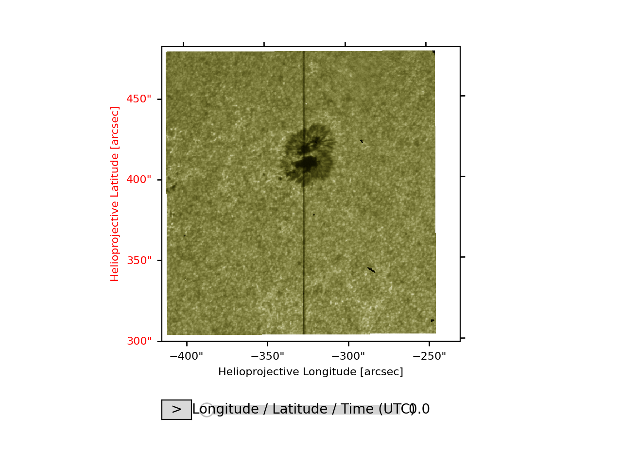
Visualizing Level 2 Data

Both the raster and slit-jaw cubes can be visualized using the plot method.

import matplotlib.pyplot as plt

iris_sji.plot()

plt.show()

(Source code, png, hires.png, pdf)

Note

We imported matplotlib.pyplot in order to create the figure.

Under the hood, irispy via ndcube via astropy using matplotlib to visualize the image meaning that plots built with irispy can be further customized using either astropy’s WCSAxes or matplotlib API.

Note that the colormap has been set by irispy based on the wavelength of the observation. This only applies to the slit-jaw images, as the raster cubes do not have a single wavelength thus the colormap is set to a default matplotlib one.

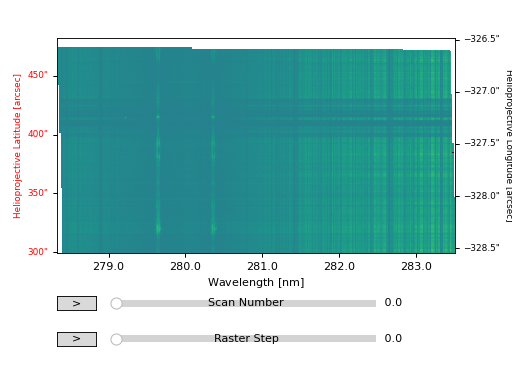
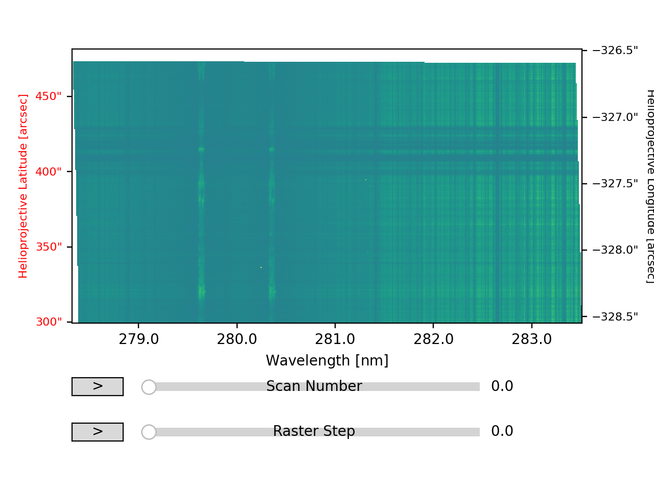
import matplotlib.pyplot as plt

raster["Mg II k 2796"].plot(vmax=255)

plt.show()

(Source code, png, hires.png, pdf)

Since they are both series of images, the plot method will automatically create a slider to scroll through the different time steps or raster steps. Furthermore, the tick and axes labels have been automatically set based on the coordinate system of the cube and are colored according to the axis direction.

Within the Tutorial Gallery, there are more examples of how to visualize the data and customize the plots.