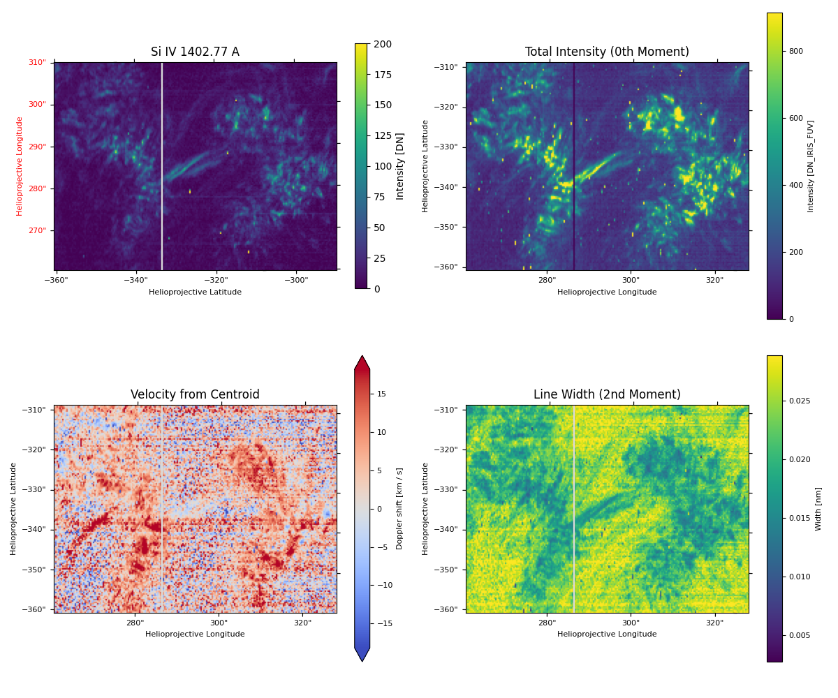
Calculate Spectral Line Moments

In this example, we are going to calculate the spectral moments from IRIS raster data. Moments provide a model-independent way to characterize spectral lines:

• 0th moment gives the total intensity

• 1st moment gives the centroid (Doppler shift)

• 2nd moment gives the line width

This is direct contrast to fitting a model to the data which is done in example Fit Spectral Models to Spectra where we fit a Gaussian to the line profile and extract the same information from the fit parameters.

import matplotlib.pyplot as plt
import numpy as np
import pooch

import astropy.units as u
from astropy.coordinates import SkyCoord, SpectralCoord
from astropy.visualization import time_support
from astropy.wcs.utils import wcs_to_celestial_frame

from sunpy.coordinates.frames import Helioprojective

from irispy.io import read_files
from irispy.utils.moments import calculate_moments

time_support()

<astropy.visualization.time.time_support.<locals>.MplTimeConverter object at 0x71f3dbaee510>

We start with getting data from the IRIS data archive.

In this case, we will use pooch to keep this example self-contained but you can download the data manually using your browser as well.

You will need to update the path to the data in the next section if you do that.

raster_filename = pooch.retrieve(
    "http://www.lmsal.com/solarsoft/irisa/data/level2_compressed/2018/01/02/20180102_153155_3610108077/iris_l2_20180102_153155_3610108077_raster.tar.gz",
    known_hash="8949562149cfa5fba067b5b102e8434b14cea3c3416dd79c06b7f6e211c61a39",
)

We will now open the data using a helper function which is designed to read all files from a single observation.

raster = read_files(raster_filename)

We will just focus on the Si IV 1403 line which we can select using a key. Then we will just plot a spectral line selected at random in space.

# There is only one complete scan, so we index that away.
si_iv_1403 = raster["Si IV 1403"][0]

# However, before we get to that, we will shrink the data cube to make it easier to work with.
iris_observer = wcs_to_celestial_frame(si_iv_1403.wcs.celestial).observer
iris_frame = Helioprojective(observer=iris_observer)
top_left = [None, SkyCoord(-290 * u.arcsec, 260 * u.arcsec, frame=iris_frame)]
bottom_right = [None, SkyCoord(-360 * u.arcsec, 310 * u.arcsec, frame=iris_frame)]
si_iv_1403 = si_iv_1403.crop(top_left, bottom_right)

/home/docs/checkouts/readthedocs.org/user_builds/irispy/conda/stable/lib/python3.13/site-packages/astropy/wcs/wcsapi/fitswcs.py:555: AstropyUserWarning: target cannot be converted to ICRS, so will not be set on SpectralCoord
  warnings.warn(

Let us just check the full field of view at the line core.

si_iv_core = 140.277 * u.nm
lower_corner = [SpectralCoord(si_iv_core), None]
upper_corner = [SpectralCoord(si_iv_core), None]
si_iv_spec_crop = si_iv_1403.crop(lower_corner, upper_corner)

/home/docs/checkouts/readthedocs.org/user_builds/irispy/conda/stable/lib/python3.13/site-packages/astropy/wcs/wcsapi/fitswcs.py:723: AstropyUserWarning: No observer defined on WCS, SpectralCoord will be converted without any velocity frame change
  warnings.warn(

Now we can calculate the spectral moments using the calculate_moments function.

This helper function automatically extracts the wavelength coordinates from the cube’s WCS and computes the moments along the spectral axis for every spatial pixel.

We will restrict the calculation to a narrow window around the rest wavelength (0.05 nm = 0.5 Å on each side) to isolate the Si IV line from its neighbors.

While wings is not required, it is often a good idea to restrict the calculation to a window around the line of interest to avoid contamination from other lines or noise in the continuum.

The same goes for rest_wavelength, which is used to calculate the velocity from the wavelength shift in the 1st moment, otherwise you get the centroid in wavelength units instead of velocity units and the same goes for the line width from the 2nd moment.

moments = calculate_moments(si_iv_1403, rest_wavelength=si_iv_core, wings=0.05 * u.nm, integrated=False)
# The return is a RasterCollection with the same form as the input cube.
intensity = moments["intensity"]
centroid = moments["centroid"]
width = moments["width"]
velocity = moments["velocity"]
velocity_width = moments["velocity_width"]

We will now visualize the moments. Note that the output is a RasterCollection which contains 2D SpectrogramCube objects with the spatial WCS preserved from the input cube.

Note that we are transposing the data arrays so they match up with the projection which is in X,Y.

fig, ax_dict = plt.subplot_mosaic(
    [["fov", "intensity"], ["velocity", "width"]],
    subplot_kw={"projection": si_iv_spec_crop.wcs},
    figsize=(12, 10),
)

si_iv_spec_crop.plot(axes=ax_dict["fov"], plot_axes=["x", "y"], vmin=0, vmax=200)
ax_dict["fov"].set_title("Si IV 1402.77 A")
fig.colorbar(ax_dict["fov"].images[0], ax=ax_dict["fov"], label="Intensity [DN]", shrink=0.8)

# 0th moment: Total intensity
amp_max = np.nanpercentile(np.abs(intensity.data), 99)
amp = ax_dict["intensity"].imshow(intensity.data.T, vmin=0, vmax=amp_max, origin="lower")
cbar = fig.colorbar(amp, ax=ax_dict["intensity"])
cbar.set_label(label=f"Intensity [{intensity.unit.to_string()}]", fontsize=8)
cbar.ax.tick_params(labelsize=8)
ax_dict["intensity"].set_title("Total Intensity (0th Moment)")

# 1st moment: Doppler velocity from centroid shift
shift_max = np.nanpercentile(np.abs(velocity.data), 95)
shift = ax_dict["velocity"].imshow(velocity.data.T, cmap="coolwarm", vmin=-shift_max, vmax=shift_max, origin="lower")
cbar = fig.colorbar(shift, ax=ax_dict["velocity"], extend="both")
cbar.set_label(label=f"Doppler shift [{velocity.unit.to_string()}]", fontsize=8)
cbar.ax.tick_params(labelsize=8)
ax_dict["velocity"].set_title("Velocity from Centroid")

# 2nd moment: Line width
wmax = np.nanpercentile(width.data, 95)
wdisp = ax_dict["width"].imshow(width.data.T, vmax=wmax, origin="lower")
cbar = fig.colorbar(wdisp, ax=ax_dict["width"])
cbar.set_label(label=f"Width [{width.unit.to_string()}]", fontsize=8)
cbar.ax.tick_params(labelsize=8)
ax_dict["width"].set_title("Line Width (2nd Moment)")

for ax in ax_dict.values():
    ax.coords[0].set_ticklabel(exclude_overlapping=True, fontsize=8)
    ax.coords[0].set_axislabel("Helioprojective Longitude", fontsize=8)
    ax.coords[1].set_ticklabel(exclude_overlapping=True, fontsize=8)
    ax.coords[1].set_axislabel("Helioprojective Latitude", fontsize=8)
fig.tight_layout()

plt.show()