Open the IRIS Aligned AIA Cubes

In this example we will show how irispy handles the AIA cubes provided by the IRIS instrument team. These cubes are aligned to the IRIS observation and are 50” larger than the IRIS FOV.

They have the same format as IRIS SJI files, so you can read them via irispy.

import matplotlib.pyplot as plt
import pooch

from irispy.io import read_files

We start with getting data from the IRIS data archive.

In this case, we will use pooch to keep this example self-contained but you can download the data manually using your browser as well.

You will need to update the path to the data in the next section if you do that.

sdo_aia_file = pooch.retrieve(
    "https://www.lmsal.com/solarsoft/irisa/data/level2_compressed/2025/05/19/20250519_165924_3640107442/iris_l2_20250519_165924_3640107442_SDO.tar.gz",
    known_hash="b77d693fa328a96aec78b4a4aa420d5b167f8f670719fce815836627ed567f42",
)

We will now open the AIA dataset.

It is provided as a compressed archive, with each AIA wavelength as a separate file.

In this example, they are:

• aia_l2_20250519_165924_3640107442_171.fits

• aia_l2_20250519_165924_3640107442_94.fits

• aia_l2_20250519_165924_3640107442_304.fits

• aia_l2_20250519_165924_3640107442_193.fits

• aia_l2_20250519_165924_3640107442_335.fits

• aia_l2_20250519_165924_3640107442_211.fits

• aia_l2_20250519_165924_3640107442_1700.fits

• aia_l2_20250519_165924_3640107442_131.fits

• aia_l2_20250519_165924_3640107442_1600.fits

# This will return a list of the AIA cubes.
aia_collection = read_files(sdo_aia_file)

Let us look at the first collection returned of the AIA cube.

print(aia_collection)

NDCollection
------------
Cube keys: ('171_THIN', '94_THIN', '304_THIN', '193_THIN', '335_THIN', '211_THIN', '1700', '131_THIN', '1600')
Number of Cubes: 9
Aligned dimensions: None
Aligned physical types: None

We will then select the 304 bandpass cube.

print(aia_collection["304_THIN"])

AIACube
-------
Observatory:
Instrument:            AIA_4
Bandpass:              304
Obs Date:              2025-05-19T16:49:29.130 -- 2025-05-19T18:00:41.133
Total Frames in Obs:   None
Obs ID:                20250519_165924_3640107442
Obs Description:
Axis Types:            [('custom:pos.helioprojective.lon', 'custom:pos.helioprojective.lat', 'time', 'custom:CUSTOM', 'custom:CUSTOM', 'custom:CUSTOM', 'custom:CUSTOM', 'custom:CUSTOM', 'custom:CUSTOM', 'custom:CUSTOM', 'custom:CUSTOM', 'custom:CUSTOM'), ('custom:pos.helioprojective.lon', 'custom:pos.helioprojective.lat'), ('custom:pos.helioprojective.lon', 'custom:pos.helioprojective.lat')]
Roll:                  -0.000345947
Cube dimensions:       (357, 381, 421)

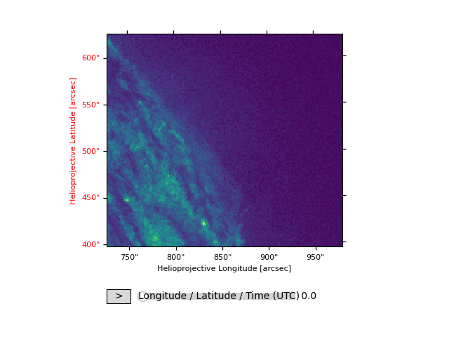
We will now plot the AIA data in the same manner as the SJI data.

You can also change the axis labels and ticks if you so desire. WCSAxes provides us an API we can use.

fig = plt.figure()
aia_collection["304_THIN"].plot(fig=fig)

plt.show()