Fit Spectral Models to Spectra - Double Gaussian Fitting

In this example, we are going to fit spectral lines from IRIS, using the raster data with a double Gaussian model. Then we will use the fitted values to calculate the Gaussian moments.

If you want to see a similar example but with a single Gaussian fit to the Si IV 1403 line, see Fit Spectral Models to Spectra. This example also has more detailed comments on the fitting process, so it may be worth looking at that example first before this one.

This is direct contrast to taking the spectral moments of the data cube, which is done in the following example, Calculate Spectral Line Moments where we calculate the spectral moments of the data cube directly.

import matplotlib.pyplot as plt
import numpy as np
import pooch

import astropy.units as u
from astropy import constants
from astropy.coordinates import SkyCoord, SpectralCoord
from astropy.modeling import models as m
from astropy.modeling.fitting import LMLSQFitter, TRFLSQFitter, parallel_fit_dask
from astropy.visualization import time_support
from astropy.wcs.utils import wcs_to_celestial_frame

from sunpy.coordinates.frames import Helioprojective

from irispy.io import read_files

time_support()

<astropy.visualization.time.time_support.<locals>.MplTimeConverter object at 0x71f3d3075a90>

We start with getting data from the IRIS data archive.

In this case, we will use pooch to keep this example self-contained but you can download the data manually using your browser as well.

You will need to update the path to the data in the next section if you do that.

raster_filename = pooch.retrieve(
    "http://www.lmsal.com/solarsoft/irisa/data/level2_compressed/2018/01/02/20180102_153155_3610108077/iris_l2_20180102_153155_3610108077_raster.tar.gz",
    known_hash="8949562149cfa5fba067b5b102e8434b14cea3c3416dd79c06b7f6e211c61a39",
)

We will now open the data using a helper function which is designed to read all files from a single observation.

We read only the Mg II k window and select the one complete scan.

raster = read_files(raster_filename, spectral_windows="Mg II k 2796")
mg_ii_k = raster["Mg II k 2796"][0]

We crop the spatial field of view to keep the example light enough for the documentation build. We will also focus on the Mg II k core, which is the part of the spectrum we are going to fit.

iris_observer = wcs_to_celestial_frame(mg_ii_k.wcs.celestial).observer
iris_frame = Helioprojective(observer=iris_observer)
top_left = [None, SkyCoord(-350 * u.arcsec, 310 * u.arcsec, frame=iris_frame)]
bottom_right = [None, SkyCoord(-290 * u.arcsec, 260 * u.arcsec, frame=iris_frame)]
mg_ii_k = mg_ii_k.crop(top_left, bottom_right)

lower_corner = [SpectralCoord(279.40, unit=u.nm), None]
upper_corner = [SpectralCoord(279.80, unit=u.nm), None]
mg_ii_k = mg_ii_k.crop(lower_corner, upper_corner)

/home/docs/checkouts/readthedocs.org/user_builds/irispy/conda/stable/lib/python3.13/site-packages/astropy/wcs/wcsapi/fitswcs.py:555: AstropyUserWarning: target cannot be converted to ICRS, so will not be set on SpectralCoord
  warnings.warn(
/home/docs/checkouts/readthedocs.org/user_builds/irispy/conda/stable/lib/python3.13/site-packages/astropy/wcs/wcsapi/fitswcs.py:723: AstropyUserWarning: No observer defined on WCS, SpectralCoord will be converted without any velocity frame change
  warnings.warn(

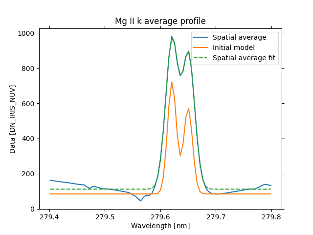
We use the spatially averaged profile to tune the initial double Gaussian model.

spatial_mean = mg_ii_k.rebin((*mg_ii_k.data.shape[:-1], 1))[0, 0, :]
spectral_axis = "em.wl"
wavelength_coords = spatial_mean.axis_world_coords(spectral_axis)[0].to(u.nm)

continuum = np.nanpercentile(spatial_mean.data, 10) * spatial_mean.unit
peak = np.nanmax(spatial_mean.data) * spatial_mean.unit
initial_model = (
    m.Const1D(amplitude=continuum)
    + m.Gaussian1D(amplitude=0.65 * peak, mean=279.621 * u.nm, stddev=0.008 * u.nm)
    + m.Gaussian1D(amplitude=0.50 * peak, mean=279.650 * u.nm, stddev=0.008 * u.nm)
)

fitter = TRFLSQFitter()
average_fit = fitter(
    initial_model,
    wavelength_coords,
    spatial_mean.data * spatial_mean.unit,
)

Now we check, the initial model and the model fitted to the average spectra.

plt.figure()
ax = spatial_mean.plot(label="Spatial average")
ax.plot(initial_model(wavelength_coords), label="Initial model")
ax.plot(average_fit(wavelength_coords), linestyle="--", label="Spatial average fit")
ax.set_title("Mg II k average profile")
plt.legend()

<matplotlib.legend.Legend object at 0x71f3d1a6c910>

We now fit the double Gaussian model to every spatial pixel.

mg_ii_model_fit = parallel_fit_dask(
    data=np.nan_to_num(mg_ii_k.data.clip(min=0)),
    data_unit=mg_ii_k.unit,
    fitting_axes=2,
    world=(wavelength_coords,),
    model=average_fit,
    fitter=LMLSQFitter(),
    scheduler="single-threaded",
)

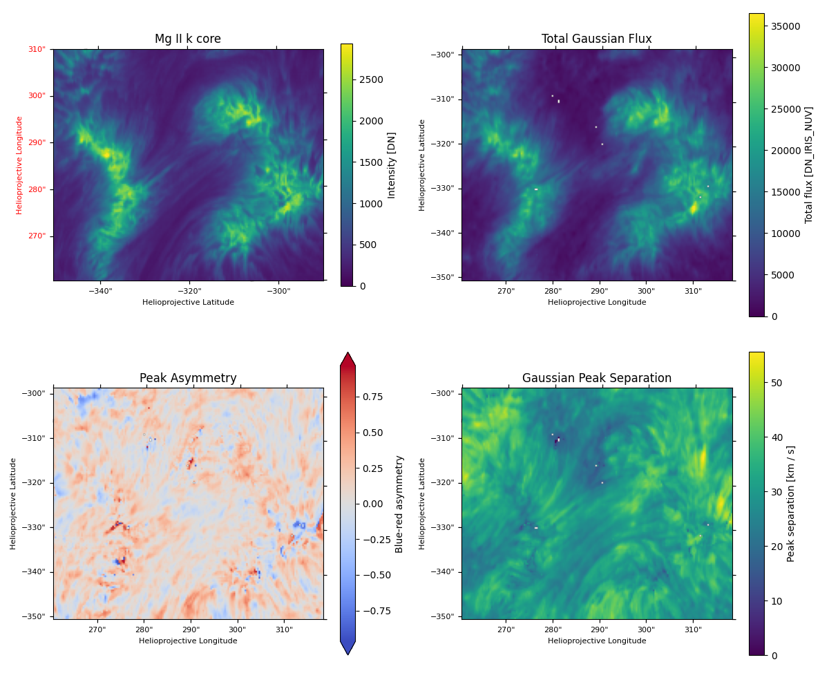
Now we will produce maps of the total fitted flux, the blue-red peak asymmetry, and the peak separation.

These maps are motivated by the Mg II h/k diagnostics described by Leenaarts et al. (2013).

In that work, the Mg II k2 peak intensities, blue-red peak imbalance, and peak separation were shown to trace chromospheric temperature, upper-chromospheric velocities, and velocity gradients. Here the two Gaussian components provide a simple fitted proxy for the k2v/k2r profile diagnostics, rather than a full radiative-transfer inversion.

mg_ii_core = 279.6351 * u.nm
line_core = mg_ii_k.crop([SpectralCoord(mg_ii_core), None], [SpectralCoord(mg_ii_core), None])
wavelength_step = np.mean(np.diff(mg_ii_k.axis_world_coords(spectral_axis)[0])).to(u.nm)

blue_flux = np.sqrt(2 * np.pi) * mg_ii_model_fit.amplitude_1 * mg_ii_model_fit.stddev_1.quantity / wavelength_step
red_flux = np.sqrt(2 * np.pi) * mg_ii_model_fit.amplitude_2 * mg_ii_model_fit.stddev_2.quantity / wavelength_step
valid_components = (
    np.isfinite(blue_flux.value) & np.isfinite(red_flux.value) & (blue_flux.value > 0) & (red_flux.value > 0)
)
total_flux = blue_flux + red_flux
with np.errstate(divide="ignore", invalid="ignore"):
    peak_asymmetry = ((blue_flux - red_flux) / total_flux).to_value(u.dimensionless_unscaled)
peak_asymmetry = np.where(np.isfinite(peak_asymmetry) & (total_flux.value > 0), peak_asymmetry, np.nan)
peak_asymmetry = np.where(valid_components, peak_asymmetry, np.nan)
component_separation = (
    np.abs(mg_ii_model_fit.mean_2.quantity.to(u.nm) - mg_ii_model_fit.mean_1.quantity.to(u.nm))
    / mg_ii_core
    * constants.c.to(u.km / u.s)
)
component_separation = np.where(valid_components, component_separation, np.nan * component_separation.unit)
total_flux = np.where(valid_components, total_flux, np.nan * total_flux.unit)

fig, ax_dict = plt.subplot_mosaic(
    [["fov", "total_flux"], ["asymmetry", "separation"]],
    subplot_kw={"projection": line_core.wcs},
    figsize=(12, 10),
)

line_core_max = np.nanpercentile(line_core.data, 99.99)
line_core.plot(axes=ax_dict["fov"], plot_axes=["x", "y"], vmin=0, vmax=line_core_max)
ax_dict["fov"].set_title("Mg II k core")
fig.colorbar(ax_dict["fov"].images[0], ax=ax_dict["fov"], label="Intensity [DN]", shrink=0.8)

flux_max = np.nanpercentile(total_flux.value, 99.99)
flux = ax_dict["total_flux"].imshow(total_flux.value.T, origin="lower", vmin=0, vmax=flux_max)
fig.colorbar(flux, ax=ax_dict["total_flux"], label=f"Total flux [{total_flux.unit.to_string()}]")
ax_dict["total_flux"].set_title("Total Gaussian Flux")

asym_max = np.nanpercentile(np.abs(peak_asymmetry), 99.99)
asymmetry = ax_dict["asymmetry"].imshow(
    peak_asymmetry.T,
    cmap="coolwarm",
    origin="lower",
    vmin=-asym_max,
    vmax=asym_max,
)
fig.colorbar(asymmetry, ax=ax_dict["asymmetry"], label="Blue-red asymmetry", extend="both")
ax_dict["asymmetry"].set_title("Peak Asymmetry")

sep_max = np.nanpercentile(np.abs(component_separation.value), 99.99)
sep = ax_dict["separation"].imshow(component_separation.value.T, origin="lower", vmin=0, vmax=sep_max)
fig.colorbar(sep, ax=ax_dict["separation"], label=f"Peak separation [{component_separation.unit.to_string()}]")
ax_dict["separation"].set_title("Gaussian Peak Separation")

for ax in ax_dict.values():
    ax.coords[0].set_ticklabel(exclude_overlapping=True, fontsize=8)
    ax.coords[0].set_axislabel("Helioprojective Longitude", fontsize=8)
    ax.coords[1].set_ticklabel(exclude_overlapping=True, fontsize=8)
    ax.coords[1].set_axislabel("Helioprojective Latitude", fontsize=8)
fig.tight_layout()

plt.show()

/home/docs/checkouts/readthedocs.org/user_builds/irispy/conda/stable/lib/python3.13/site-packages/astropy/wcs/wcsapi/fitswcs.py:555: AstropyUserWarning: target cannot be converted to ICRS, so will not be set on SpectralCoord
  warnings.warn(
/home/docs/checkouts/readthedocs.org/user_builds/irispy/conda/stable/lib/python3.13/site-packages/astropy/wcs/wcsapi/fitswcs.py:723: AstropyUserWarning: No observer defined on WCS, SpectralCoord will be converted without any velocity frame change
  warnings.warn(