Crop IRIS SJI

In this example we will show crop a IRIS dataset and the particularity of the crop operation.

import matplotlib.pyplot as plt
import pooch

import astropy.units as u
from astropy.coordinates import SkyCoord
from astropy.wcs.utils import wcs_to_celestial_frame

from irispy.io import read_files
from irispy.obsid import ObsID

We start with getting data from the IRIS data archive.

In this case, we will use pooch to keep this example self-contained but you can download the data manually using your browser as well.

You will need to update the path to the data in the next section if you do that.

sji_filename = pooch.retrieve(
    "http://www.lmsal.com/solarsoft/irisa/data/level2_compressed/2014/09/19/20140919_051712_3860608353/iris_l2_20140919_051712_3860608353_SJI_2832_t000.fits.gz",
    known_hash="7ec0f3d63d97bc7620675c78fb6c670ef5b4249d31ef7818435b629c04b72f60",
)

We will now open the data using a helper function which is designed to read all files from a single observation.

sji_2832 = read_files(sji_filename)

Printing will give us an overview of the file.

print(sji_2832)
# ``.meta`` contains the entire FITS header from the primary HDU.
# Since it is very long, we won't actually print it here.
# print(sji_2832.meta)

SJICube
-------
Observatory:           IRIS
Instrument:            SJI
Bandpass:              2832.0
Obs Date:              2014-09-19T05:17:31.110 -- 2014-09-19T07:13:24.610
Total Frames in Obs:   None
Obs ID:                3860608353
Obs Description:       Large sit-and-stare 0.3x120 1s  C II   Mg II h/k   Mg II w s Deep x
Axis Types:            [('custom:pos.helioprojective.lon', 'custom:pos.helioprojective.lat', 'time', 'custom:CUSTOM', 'custom:CUSTOM', 'custom:CUSTOM', 'custom:CUSTOM', 'custom:CUSTOM', 'custom:CUSTOM', 'custom:CUSTOM', 'custom:CUSTOM', 'custom:CUSTOM'), ('custom:pos.helioprojective.lon', 'custom:pos.helioprojective.lat'), ('custom:pos.helioprojective.lon', 'custom:pos.helioprojective.lat')]
Roll:                  45.0001
Cube dimensions:       (65, 387, 364)

Can’t remember what is OBSID 3860608353?

irispy has an utility function that will provide more information.

print(ObsID(sji_2832.meta["OBSID"]))

IRIS OBS ID 3860608353
----------------------
Description:                      Large sit-and-stare 0.3x120 1s
SJI filters:                        C II   Mg II h/k   Mg II w s
SJI field of view:                                       120x120
Exposure time:                                               8.0 s
Binning:                               Spatial x 2, Spectral x 2
FUV binning:                         FUV spectrally rebinned x 4
SJI cadence:                                 SJI cadence default
Compression:                                 Default compression
Linelist:                                       Flare linelist 1

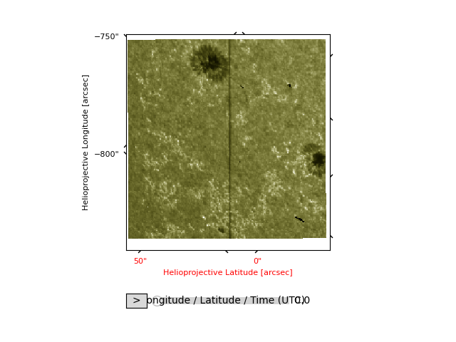
Now, we will plot the SJI. By default, irispy will color the spatial axes.

# This is an animation
sji_2832.plot()

<irispy.visualization.IRISArrayAnimatorWCS object at 0x71f3d1a6ee90>

We also have the option of going directly to an individual scan.

sji_45 = sji_2832[45]
print(sji_45)

SJICube
-------
Observatory:           IRIS
Instrument:            SJI
Bandpass:              2832.0
Obs Date:              2014-09-19T06:39:00.270 -- None
Total Frames in Obs:   None
Obs ID:                3860608353
Obs Description:       Large sit-and-stare 0.3x120 1s  C II   Mg II h/k   Mg II w s Deep x
Axis Types:            [('custom:pos.helioprojective.lon', 'custom:pos.helioprojective.lat'), ('custom:pos.helioprojective.lon', 'custom:pos.helioprojective.lat')]
Roll:                  45.0001
Cube dimensions:       (387, 364)

We need to get the coordinate frame for the IRIS data. While this is stored in the WCS, getting a coordinate frame is a little more involved. We will use this to do a cutout later on.

sji_frame = wcs_to_celestial_frame(sji_45.basic_wcs)
bbox = [
    SkyCoord(-750 * u.arcsec, 90 * u.arcsec, frame=sji_frame),
    SkyCoord(-750 * u.arcsec, 95 * u.arcsec, frame=sji_frame),
    SkyCoord(-700 * u.arcsec, 90 * u.arcsec, frame=sji_frame),
    SkyCoord(-700 * u.arcsec, 95 * u.arcsec, frame=sji_frame),
]

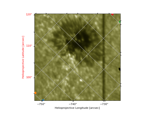
This dataset has a peculiarity: the observation has a 45 degree roll. The image does not have a 45 degree rotation because plotting shows the data in the way they are written in the file. We will a coordinate grid to make this clear.

You can also change the axis labels and ticks if you so desire. WCSAxes provides us an API we can use.

Now, let us cut out the top sunspot.

We need to specify the corners for the cut (note the coordinate order is the same as the plotted image). Be aware that crop works in the default N/S frame, so it will crop along those axes where as the data is rotated. You will also need to create a proper bounding box, with 4 corners.

crop will return you the smallest bounding box which contains those 4 points which we can see when we overlay the points we give it. So despite the bounding box being the incorrect location, it returns the cutout we want.

sji_cutout = sji_45.crop(*bbox)

plt.figure()
ax = sji_cutout.plot()
# Plot each corner of the box
[ax.plot_coord(coord, "o") for coord in bbox]
# You have to specify the grid type to be contours for WCSAxes to plot it correctly.
# This is due to a quirk of how gWCS interacts with WCSAxes.
ax.coords.grid(grid_type="contours")

plt.show()