Fit Spectral Models to Spectra

In this example, we are going to fit Si IV 1403 from IRIS with a single Gaussian. Then we will use the fitted values to calculate the Gaussian moments.

This is direct contrast to taking the spectral moments of the data cube, which is done in the following example, Calculate Spectral Line Moments where we calculate the spectral moments of the data cube directly.

If you want to see a similar example but with a double Gaussian fit to the Mg II k line, see Fit Spectral Models to Spectra - Double Gaussian Fitting.

import shutil
from pathlib import Path

import matplotlib.pyplot as plt
import numpy as np
import pooch

import astropy.units as u
from astropy import constants
from astropy.coordinates import SkyCoord, SpectralCoord
from astropy.modeling import models as m
from astropy.modeling.fitting import LMLSQFitter, TRFLSQFitter, parallel_fit_dask
from astropy.visualization import time_support
from astropy.wcs.utils import wcs_to_celestial_frame

from sunpy.coordinates.frames import Helioprojective

from irispy.io import read_files

time_support()

<astropy.visualization.time.time_support.<locals>.MplTimeConverter object at 0x71f3db7ca120>

We start with getting data from the IRIS data archive.

In this case, we will use pooch to keep this example self-contained but you can download the data manually using your browser as well.

You will need to update the path to the data in the next section if you do that.

raster_filename = pooch.retrieve(
    "http://www.lmsal.com/solarsoft/irisa/data/level2_compressed/2018/01/02/20180102_153155_3610108077/iris_l2_20180102_153155_3610108077_raster.tar.gz",
    known_hash="8949562149cfa5fba067b5b102e8434b14cea3c3416dd79c06b7f6e211c61a39",
)

We will now open the data using a helper function which is designed to read all files from a single observation. We read only the Si IV 1403 window and select the one complete scan.

raster = read_files(raster_filename, spectral_windows="Si IV 1403")
si_iv_1403 = raster["Si IV 1403"][0]

However, before we get to fitting, we will shrink the data cube to make it easier to work with. This is done primarily to speed up the fitting process on the online documentation build.

iris_observer = wcs_to_celestial_frame(si_iv_1403.wcs.celestial).observer
iris_frame = Helioprojective(observer=iris_observer)
top_left = [None, SkyCoord(-290 * u.arcsec, 260 * u.arcsec, frame=iris_frame)]
bottom_right = [None, SkyCoord(-360 * u.arcsec, 310 * u.arcsec, frame=iris_frame)]
si_iv_1403 = si_iv_1403.crop(top_left, bottom_right)

/home/docs/checkouts/readthedocs.org/user_builds/irispy/conda/stable/lib/python3.13/site-packages/astropy/wcs/wcsapi/fitswcs.py:555: AstropyUserWarning: target cannot be converted to ICRS, so will not be set on SpectralCoord
  warnings.warn(

Let us just get the full field of view at the line core.

si_iv_core = 140.277 * u.nm
lower_corner = [SpectralCoord(si_iv_core), None]
upper_corner = [SpectralCoord(si_iv_core), None]
si_iv_spec_crop = si_iv_1403.crop(lower_corner, upper_corner)

/home/docs/checkouts/readthedocs.org/user_builds/irispy/conda/stable/lib/python3.13/site-packages/astropy/wcs/wcsapi/fitswcs.py:723: AstropyUserWarning: No observer defined on WCS, SpectralCoord will be converted without any velocity frame change
  warnings.warn(

We will want to make two rebinned cubes from the full raster, one summed along the wavelength dimension and one of the spectra averaged over all spatial pixels.

wl_sum = si_iv_1403.rebin((1, 1, si_iv_1403.data.shape[-1]), operation=np.sum)[0]
spatial_mean = si_iv_1403.rebin((*si_iv_1403.data.shape[:-1], 1))[0, 0, :]
wavelength_coords = spatial_mean.axis_world_coords("em.wl")[0].to(u.nm)

Now we can create a model for this spectra.

initial_model = m.Const1D(amplitude=2 * si_iv_1403.unit) + m.Gaussian1D(
    amplitude=8 * si_iv_1403.unit, mean=si_iv_core, stddev=0.005 * u.nm
)

To improve our initial conditions we now fit the initial model to the spatially averaged spectra. To do this we use the ndcube.NDCube.axis_world_coords method of NDCube which returns all, or a subset of the world coordinates along however many array axes they are correlated with. So in this case we get the wavelength dimension which only returns a single astropy.coordinates.SpectralCoord object corresponding to the first array dimension of the cube.

fitter = TRFLSQFitter()
average_fit = fitter(
    initial_model,
    wavelength_coords,
    spatial_mean.data * spatial_mean.unit,
)

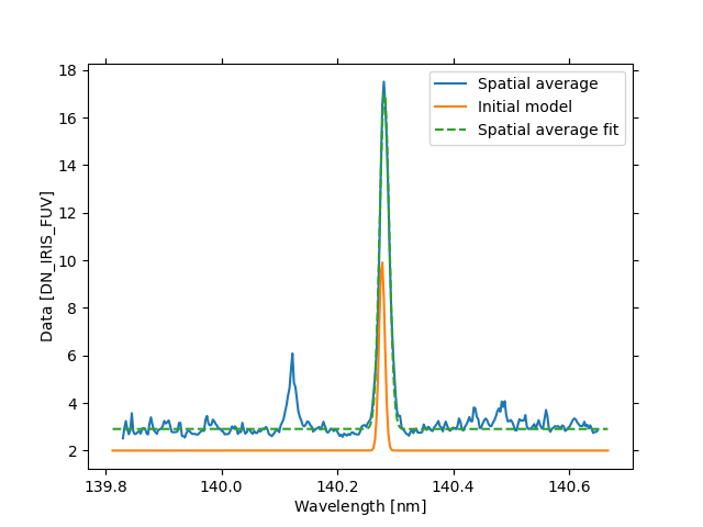
Now we check, the initial model and the model fitted to the average spectra.

fig = plt.figure()
ax = spatial_mean.plot(label="Spatial average")
ax.plot(initial_model(wavelength_coords), label="Initial model")
ax.plot(average_fit(wavelength_coords), linestyle="--", label="Spatial average fit")
plt.legend()

<matplotlib.legend.Legend object at 0x71f3d1a6c550>

The function parallel_fit_dask will map a model to each element of a cube along one (or more) “fitting axes”, in this case our fitting axis is our wavelength axis (array axis -1). So we want to fit each slice of the data array along the 3rd axis.

The key arguments to the parallel_fit_dask function are:

• A data array: This can be a numpy array or a dask array, or a NDData (or subclass like NDCube)

  object. If it’s a NDData object then the data, wcs, mask, data_unit and uncertainty are all extracted from the NDData object and used in place of their respective keyword arguments.

• A model to fit

• A fitter instance.

• The fitting axis (or axes).

What is returned from parallel_fit_dask is a model with array parameters with the shape of the non-fitting axes of the data.

# We want to do some basic data sanitization.
# Remove negative values and set them to zero and remove non-finite values.
filtered_data = np.where(si_iv_1403.data < 0, 0, si_iv_1403.data)
filtered_data = np.where(np.isfinite(filtered_data), filtered_data, 0)

Before we fit the data cube, I want to briefly talk about errors during the fitting process.

It is possible that the fitting process will fail for some pixels. This can be for a variety of reasons, but most commonly it is because the fitting algorithm cannot converge to a solution. When this happens the fitting algorithm will raise a warning/exception. However, when using parallel_fit_dask, these warnings/exceptions are caught and not raised. Instead, the parameter values for that pixel are set to NaN.

If you want to diagnose why, you can set the diagnostics and diagnostics_path keyword arguments.

diag_path = Path("./diag")
shutil.rmtree(diag_path, ignore_errors=True)

# We can therefore fit the cube
iris_model_fit = parallel_fit_dask(
    data=filtered_data,
    data_unit=si_iv_1403.unit,
    fitting_axes=2,
    # We are fitting along the wavelength axis, so we need to provide the world coordinates
    # along this axis. The input has to be a tuple of length equal to the number of fitting axes.
    world=(wavelength_coords,),
    model=average_fit,
    # You can replace this with TRFLSQFitter, LMLSQFitter is faster in a single thread
    # which is why we use it here in this example.
    fitter=LMLSQFitter(),
    scheduler="single-threaded",
    # See above for the error handling discussion
    diagnostics="error",
    diagnostics_path=diag_path,
)

Note that this example is done in a single thread. If you want to use multiple cores. You can create a dask client and pass it to the parallel_fit_dask function.

For example:

from dask.distributed import Client

client = Client()

Then pass this to the parallel_fit_dask function by replacing scheduler line above with:

scheduler=client,

Now let us check if there were any errors during the fitting process. In this example there were none, but if there were you would find them in the “diag” folder.

errors = [p.read_text() for p in diag_path.rglob("error.log")]
print(f"{len(errors)} errors occurred")
if errors:
    print("First error is:")
    print(errors[0])

0 errors occurred

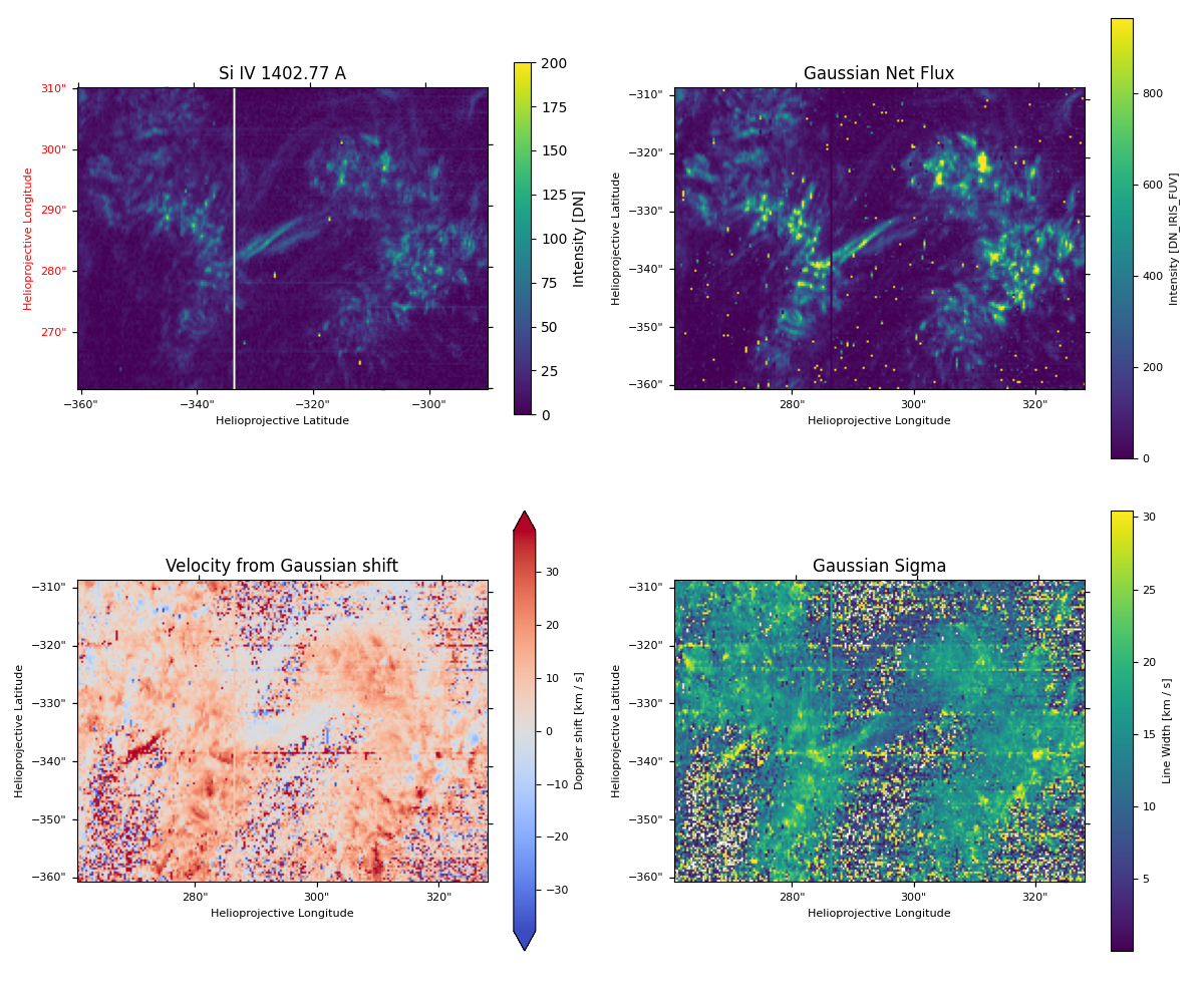
Let us see the fitted output. The model parameters are now 2D arrays with the same shape as the spatial dimensions of the data cube.

Below is a lot of custom code to make a decent looking plot.

We also need to convert the fitted parameters into physical quantities.

# Note that we are transposing the data arrays so they match up with the projection which is in X,Y.
fig, ax_dict = plt.subplot_mosaic(
    [["fov", "net_flux"], ["velocity", "sigma"]],
    subplot_kw={"projection": si_iv_spec_crop.wcs},
    figsize=(12, 10),
)

si_iv_spec_crop.plot(axes=ax_dict["fov"], plot_axes=["x", "y"], vmin=0, vmax=200)
ax_dict["fov"].set_title("Si IV 1402.77 A")
fig.colorbar(ax_dict["fov"].images[0], ax=ax_dict["fov"], label="Intensity [DN]", shrink=0.8)

net_flux = (
    np.sqrt(2 * np.pi)
    * (iris_model_fit.amplitude_1)
    * iris_model_fit.stddev_1.quantity
    / np.mean(si_iv_1403.axis_world_coords("wl")[0][1:] - si_iv_1403.axis_world_coords("wl")[0][:-1]).to(u.nm)
)
amp_max = np.nanpercentile(np.abs(net_flux.value), 99)
amp = ax_dict["net_flux"].imshow(net_flux.value.T, vmin=0, vmax=amp_max, origin="lower")
cbar = fig.colorbar(amp, ax=ax_dict["net_flux"])
cbar.set_label(label=f"Intensity [{net_flux.unit.to_string()}]", fontsize=8)
cbar.ax.tick_params(labelsize=8)
ax_dict["net_flux"].set_title("Gaussian Net Flux")

core_shift = ((iris_model_fit.mean_1.quantity.to(u.nm)) - si_iv_core) / si_iv_core * (constants.c.to(u.km / u.s))
shift_max = np.nanpercentile(np.abs(core_shift.value), 95)
shift = ax_dict["velocity"].imshow(core_shift.value.T, cmap="coolwarm", vmin=-shift_max, vmax=shift_max)
cbar = fig.colorbar(shift, ax=ax_dict["velocity"], extend="both")
cbar.set_label(label=f"Doppler shift [{core_shift.unit.to_string()}]", fontsize=8)
cbar.ax.tick_params(labelsize=8)
ax_dict["velocity"].set_title("Velocity from Gaussian shift")

sigma = (iris_model_fit.stddev_1.quantity.to(u.nm)) / si_iv_core * (constants.c.to(u.km / u.s))
# We make any negative values nan for the purpose of the color scale.
sigma = np.where(sigma < 0, np.nan, sigma)
line_max = np.nanpercentile(np.abs(sigma.value), 95)
line = ax_dict["sigma"].imshow(sigma.value.T, vmax=line_max)
cbar = fig.colorbar(line, ax=ax_dict["sigma"])
cbar.set_label(label=f"Line Width [{sigma.unit.to_string()}]", fontsize=8)
cbar.ax.tick_params(labelsize=8)
ax_dict["sigma"].set_title("Gaussian Sigma")

for ax in ax_dict.values():
    ax.coords[0].set_ticklabel(exclude_overlapping=True, fontsize=8)
    ax.coords[0].set_axislabel("Helioprojective Longitude", fontsize=8)
    ax.coords[1].set_ticklabel(exclude_overlapping=True, fontsize=8)
    ax.coords[1].set_axislabel("Helioprojective Latitude", fontsize=8)
fig.tight_layout()

plt.show()

/home/docs/checkouts/readthedocs.org/user_builds/irispy/conda/stable/lib/python3.13/site-packages/astropy/wcs/wcsapi/fitswcs.py:555: AstropyUserWarning: target cannot be converted to ICRS, so will not be set on SpectralCoord
  warnings.warn(
/home/docs/checkouts/readthedocs.org/user_builds/irispy/conda/stable/lib/python3.13/site-packages/astropy/wcs/wcsapi/fitswcs.py:555: AstropyUserWarning: target cannot be converted to ICRS, so will not be set on SpectralCoord
  warnings.warn(