Study umbral flashes

In this tutorial, we are going to work with IRIS data to study an example of a dynamical phenomena called umbral flashes.

import matplotlib.dates as mdates
import matplotlib.pyplot as plt
import pooch

import astropy.units as u
from astropy.coordinates import SpectralCoord
from astropy.visualization import time_support

from irispy.io import read_files

time_support()

<astropy.visualization.time.time_support.<locals>.MplTimeConverter object at 0x71f3dbaee510>

We start with getting data from the IRIS data archive.

In this case, we will use pooch to keep this example self-contained but you can download the data manually using your browser as well.

You will need to update the path to the data in the next section if you do that.

raster_filename = pooch.retrieve(
    "http://www.lmsal.com/solarsoft/irisa/data/level2_compressed/2013/09/02/20130902_163935_4000255147/iris_l2_20130902_163935_4000255147_raster.tar.gz",
    known_hash="445c495cb6e4bdd8b563b318589691e3f4da79ee0e507d5ea587f1bd995fcb22",
)
sji_filename = pooch.retrieve(
    "http://www.lmsal.com/solarsoft/irisa/data/level2_compressed/2013/09/02/20130902_163935_4000255147/iris_l2_20130902_163935_4000255147_SJI_1400_t000.fits.gz",
    known_hash="1f424de4420b729385e81b00df4ba4d868a121486686f17cd1ecdbe7754ee78b",
)

We will now open the data using a helper function which is designed to read all files from a single observation.

# Since this is a large dataset, we will use memory mapping to read the data values
# directly from the FITS files without loading them into memory.

raster = read_files(raster_filename, memmap=True)
sji_1400 = read_files(sji_filename, memmap=True)

We are after the Mg II k and C II lines, which we can select using keys. Then we will produce a space-time image of the Mg II k3 line.

mg_ii = raster["Mg II k 2796"][0]
c_ii = raster["C II 1336"][0]

# Instead of using a pixel index, we can crop the data in wavelength space.
lower_corner = [SpectralCoord(279.63, unit=u.nm), None]
upper_corner = [SpectralCoord(279.63, unit=u.nm), None]
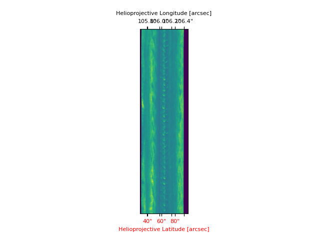
mg_crop = mg_ii.crop(lower_corner, upper_corner)

fig = plt.figure()
ax = fig.add_subplot(111, projection=mg_crop.wcs)
mg_crop.plot(axes=ax)

/home/docs/checkouts/readthedocs.org/user_builds/irispy/conda/stable/lib/python3.13/site-packages/astropy/wcs/wcsapi/fitswcs.py:555: AstropyUserWarning: target cannot be converted to ICRS, so will not be set on SpectralCoord
  warnings.warn(
/home/docs/checkouts/readthedocs.org/user_builds/irispy/conda/stable/lib/python3.13/site-packages/astropy/wcs/wcsapi/fitswcs.py:723: AstropyUserWarning: No observer defined on WCS, SpectralCoord will be converted without any velocity frame change
  warnings.warn(

<WCSAxes: >

The middle section between 60”-75” is on the umbra of a sunspot, even though it is not obvious from this image. One can see very clearly the umbral oscillations, with a clear regular pattern of dark/bright streaks.

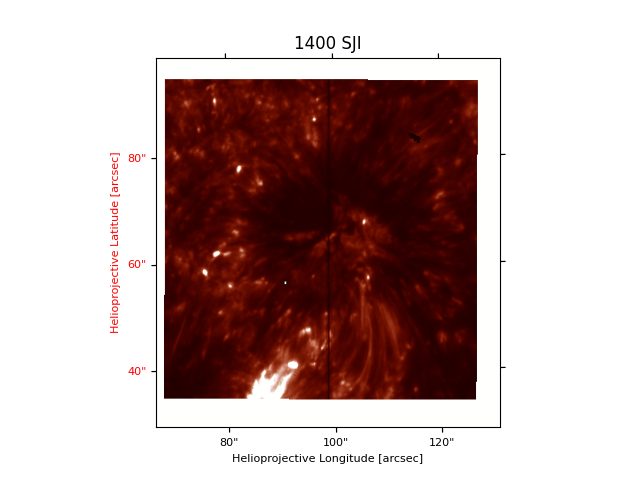
Let us now load the 1400 SJI for context.

plt.figure()
sji_1400[0].plot(vmin=-32000, vmax=-30000)
plt.title("1400 SJI")

Text(0.5, 1.0, '1400 SJI')

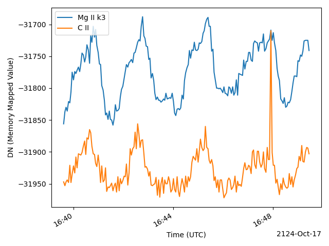
The slit pixel, “220” is a location on the sunspot’s umbra. Let us plot the k3 intensity (spectral pixel 103 of mg_ii) and the core of the brightest C II line (spectral pixel 90 of c_ii) vs time in minutes (showing first ~10 minutes only)

mg_ii_times = mg_ii.time[:200]
c_ii_times = c_ii.time[:200]

plt.figure()
plt.plot(mg_ii_times, mg_ii.data[:200, 220, 103], label="Mg II k3")
(ax,) = plt.plot(c_ii_times, c_ii.data[:200, 220, 90], label="C II")
plt.legend()
plt.ylabel("DN (Memory Mapped Value)")
plt.xlabel("Time (UTC)")
ax.axes.xaxis.set_major_formatter(mdates.ConciseDateFormatter(ax.axes.xaxis.get_major_locator()))
# Rotates and right-aligns the x labels so they don't crowd each other.
for label in ax.axes.get_xticklabels(which="major"):
    label.set(rotation=30, horizontalalignment="right")

plt.tight_layout()

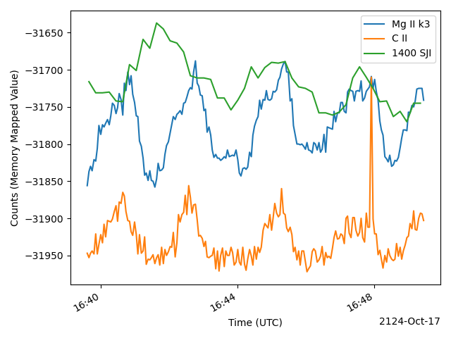
Imagine now you wanted to compare these oscillations with the intensity from the SJI. The SJI images are typically taken at a different cadence, so you need get the corresponding times for the 1400 SJI.

We will take the first 50 to cut down on the size of the data for this example.

times_sji = sji_1400.time[:50]

Now we can plot both spectral lines and SJI for a pixel close to the slit at the same Y position (pre-worked out to be at index 220).

plt.figure()
plt.plot(mg_ii_times, mg_ii.data[:200, 220, 103], label="Mg II k3")
plt.plot(c_ii_times, c_ii.data[:200, 220, 90], label="C II")
(ax,) = plt.plot(times_sji, sji_1400.data[:50, 190, 220], label="1400 SJI")
plt.legend()
plt.ylabel("Counts (Memory Mapped Value)")
plt.xlabel("Time (UTC)")
ax.axes.xaxis.set_major_formatter(mdates.ConciseDateFormatter(ax.axes.xaxis.get_major_locator()))
# Rotates and right-aligns the x labels so they don't crowd each other.
for label in ax.axes.get_xticklabels(which="major"):
    label.set(rotation=30, horizontalalignment="right")

plt.tight_layout()

plt.show()

You are now ready to explore all the correlations, anti-correlations, and phase differences.