Produce Mg II Dopplergrams

In this example, we are going to produce a Dopplergram for the Mg II k line from a 400-step raster. The Dopplergram is obtained by subtracting the intensities at symmetrical velocity shifts from the line core (e.g., ±50 km/s).

import tarfile

import matplotlib.pyplot as plt
import numpy as np
import pooch
from scipy.interpolate import make_interp_spline

import astropy.units as u
from astropy import constants
from astropy.coordinates import SpectralCoord
from astropy.io import fits

from irispy.io import read_files
from irispy.utils import image_clipping

We start with getting data from the IRIS data archive.

In this case, we will use pooch to keep this example self-contained but you can download the data manually using your browser as well.

You will need to update the path to the data in the next section if you do that.

iris_raster_tar = pooch.retrieve(
    "http://www.lmsal.com/solarsoft/irisa/data/level2_compressed/2014/07/08/20140708_114109_3824262996/iris_l2_20140708_114109_3824262996_raster.tar.gz",
    known_hash="21cff86fd0064936ce6807b1334ea1d3d50f3d358e5888810fba8e9bc1118567",
)

We will now open the data using a helper function which is designed to read all files from a single observation.

Since this is a large dataset, we will use memory mapping to read the data values directly from the FITS files without loading them into memory.

raster = read_files(iris_raster_tar, memmap=True)

We are after the Mg II k window, which we can select using a key.

mg_ii = raster["Mg II k 2796"][0]
(mg_wave,) = mg_ii.axis_world_coords("wl")

/home/docs/checkouts/readthedocs.org/user_builds/irispy/conda/stable/lib/python3.13/site-packages/astropy/wcs/wcsapi/fitswcs.py:555: AstropyUserWarning: target cannot be converted to ICRS, so will not be set on SpectralCoord
  warnings.warn(

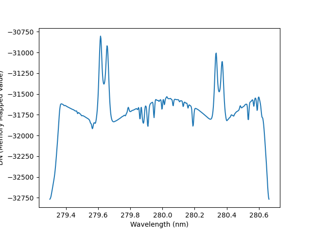
We will plot the spatially averaged spectrum:

plt.figure()
plt.plot(mg_wave.to("nm"), mg_ii.data.mean((0, 1)))
plt.ylabel("DN (Memory Mapped Value)")
plt.xlabel("Wavelength (nm)")

Text(0.5, 23.52222222222222, 'Wavelength (nm)')

This very large dense raster took more than three hours to complete across the 400 scans (with 30 s exposures), which means that the spacecraft’s orbital velocity changes during the observations. This means that any calibration will need to correct for those shifts.

To better understand the orbital velocity problem, let us look at how the line intensity varies for a strong Mn I line at around 280.2 nm, in between the Mg II k and h lines.

For this dataset, the line core of this line falls around 280.2 nm. We crop in wavelength space.

lower_corner = [SpectralCoord(280.2, unit=u.nm), None]
upper_corner = [SpectralCoord(280.2, unit=u.nm), None]
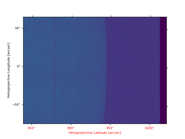
mg_crop = mg_ii.crop(lower_corner, upper_corner)
# We will "crunch" the image a bit using the aspect ratio.
mg_crop.plot(aspect="auto")

/home/docs/checkouts/readthedocs.org/user_builds/irispy/conda/stable/lib/python3.13/site-packages/astropy/wcs/wcsapi/fitswcs.py:723: AstropyUserWarning: No observer defined on WCS, SpectralCoord will be converted without any velocity frame change
  warnings.warn(

<WCSAxes: >

You can see a regular bright-dark pattern along the x-axis, an indication that the intensities are not taken at the same position in the line because of wavelength shifts. The shifts are caused by the orbital velocity changes, and we can find these in the auxiliary metadata which are to be found in the extension past the “last” window in the FITS file.

# astropy.io.fits does not support opening tar files, so we need to extract.
with tarfile.open(iris_raster_tar, "r:gz") as tar_iris_file:
    tar_iris_file.extractall("./", filter="data")

# We know ahead of time what the filename is.
raster_filename = "iris_l2_20140708_114109_3824262996_raster_t000_r00000.fits"

# The information we need is in the auxiliary data, which is stored in an
# extension past the last  window. It is always the second to last extension.
aux_data = fits.getdata(raster_filename, -2)
aux_header = fits.getheader(raster_filename, -2)
v_obs = aux_data[:, aux_header["OBS_VRIX"]] * u.m / u.s
# Convert to km/s as the data is in m/s
v_obs = v_obs.to("km/s")

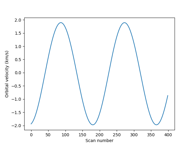
plt.figure()
plt.plot(v_obs)
plt.ylabel("Orbital velocity (km/s)")
plt.xlabel("Scan number")

Text(0.5, 23.52222222222222, 'Scan number')

To look at intensities at any given scan we only need to subtract this velocity shift from the wavelength scale, but to look at the whole image at a given wavelength we must interpolate the original data to take this shift into account. Here is a way to do it (note that array dimensions apply to this specific example).

c = constants.c.to("km/s")
mn_i_wavelength = 280.2 * u.nm
wave_shift = -v_obs * mn_i_wavelength / c
# Linear interpolation in wavelength, for each scan
for i in range(mg_ii.data.shape[0]):
    shifted_data = make_interp_spline(
        (mg_wave - wave_shift[i]).to_value(u.nm),
        mg_ii.data[i, :, :],
        k=1,
        axis=-1,
    )(mg_wave.to_value(u.nm), extrapolate=False)
    mg_ii.data[i, :, :] = np.nan_to_num(shifted_data, nan=0.0)

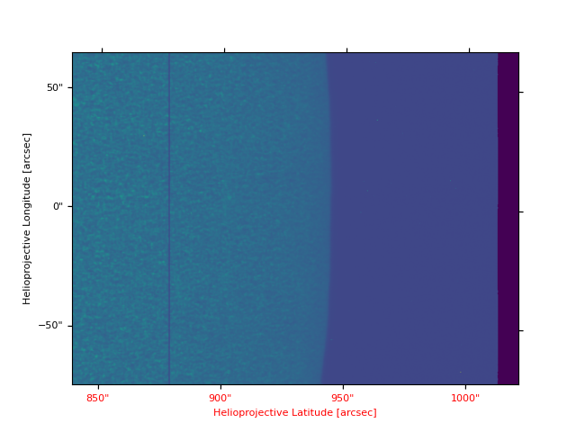
Now we can plot the shifted data to see that the large scale shifts have disappeared

plt.figure()
# Since we changed the underlying data, we need to re-crop
mg_crop = mg_ii.crop(lower_corner, upper_corner)
# We will "crunch" the image a bit using the aspect ratio.
mg_crop.plot(aspect="auto")

/home/docs/checkouts/readthedocs.org/user_builds/irispy/conda/stable/lib/python3.13/site-packages/astropy/wcs/wcsapi/fitswcs.py:555: AstropyUserWarning: target cannot be converted to ICRS, so will not be set on SpectralCoord
  warnings.warn(
/home/docs/checkouts/readthedocs.org/user_builds/irispy/conda/stable/lib/python3.13/site-packages/astropy/wcs/wcsapi/fitswcs.py:723: AstropyUserWarning: No observer defined on WCS, SpectralCoord will be converted without any velocity frame change
  warnings.warn(

<WCSAxes: >

Some residual shift remains, but we will not correct for it here. A more elaborate correction can be obtained by the IDL routine iris_prep_wavecorr_l2, but this has not yet been ported to Python see the IDL version of this tutorial for more details.

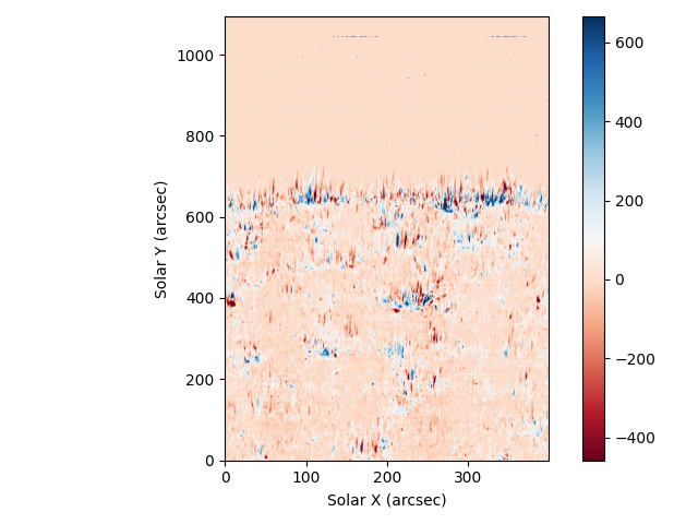
We can use the calibrated data for example to calculate Dopplergrams. A Dopplergram is here defined as the difference between the intensities at two wavelength positions at the same (and opposite) distance from the line core. For example, at +/- 50 km/s from the Mg II k3 core. To do this, let us first calculate a velocity scale for the k line and find the indices of the -50 and +50 km/s velocity positions (here using the convention of negative velocities for up flows):

mg_k_centre = 279.6351 * u.nm
pos = 50 * u.km / u.s  # Around the line centre
velocity = (mg_wave - mg_k_centre) * c / mg_k_centre
index_p = np.argmin(np.abs(velocity - pos))
index_m = np.argmin(np.abs(velocity + pos))
doppler = mg_ii.data[..., index_m] - mg_ii.data[..., index_p]

And now we can plot this as before (intensity units are again arbitrary because of the unscaled DNs).

vmin, vmax = image_clipping(doppler)
plt.figure()
plt.imshow(
    doppler.T,
    cmap="RdBu",
    origin="lower",
    aspect=0.5,
    vmin=vmin,
    vmax=vmax,
)
plt.colorbar()
plt.xlabel("Solar X (arcsec)")
plt.ylabel("Solar Y (arcsec)")
plt.tight_layout()

plt.show()