Note
Go to the end to download the full example code.
Manipulate spectrograph data#
In this example, we will showcase how to open, crop and plot IRIS spectrograph data.
import matplotlib.pyplot as plt
import numpy as np
import pooch

import astropy.units as u
from astropy.coordinates import SkyCoord, SpectralCoord
from astropy.visualization import quantity_support
from astropy.wcs.utils import wcs_to_celestial_frame

from sunpy.coordinates.frames import Helioprojective

from irispy.io import read_files

quantity_support()
<astropy.visualization.units.quantity_support.<locals>.MplQuantityConverter object at 0x71f3f162a900>
We start with getting data from the IRIS data archive.
In this case, we will use pooch to keep this example self-contained
but you can download the data manually using your browser as well.
You will need to update the path to the data in the next section if you do that.
raster_filename = pooch.retrieve(
    "http://www.lmsal.com/solarsoft/irisa/data/level2_compressed/2018/01/02/20180102_153155_3610108077/iris_l2_20180102_153155_3610108077_raster.tar.gz",
    known_hash="8949562149cfa5fba067b5b102e8434b14cea3c3416dd79c06b7f6e211c61a39",
)
We will now open the data using a helper function which is designed to read all files from a single observation.
raster = read_files(raster_filename)
Let us now explore what was returned.
Provides an overview of the Spectrograph object
print(raster)
Raster Collection
-----------------
Spectral Windows (cube keys): (np.str_('C II 1336'), np.str_('O I 1356'), np.str_('Si IV 1394'), np.str_('Si IV 1403'), np.str_('2832'), np.str_('2814'), np.str_('Mg II k 2796'))
Number of Cubes: 7
Aligned dimensions: [1 320 548]
Aligned physical types: [('meta.obs.sequence',), ('custom:pos.helioprojective.lat', 'custom:pos.helioprojective.lon', 'time'), ('custom:pos.helioprojective.lat', 'custom:pos.helioprojective.lon')]
Will give us all the keys that corresponds to all the wavelength windows.
print(raster.keys())
dict_keys([np.str_('C II 1336'), np.str_('O I 1356'), np.str_('Si IV 1394'), np.str_('Si IV 1403'), np.str_('2832'), np.str_('2814'), np.str_('Mg II k 2796')])
We can get the Mg II k window:
mg_ii = raster["Mg II k 2796"]
print(mg_ii)
/home/docs/checkouts/readthedocs.org/user_builds/irispy/conda/stable/lib/python3.13/site-packages/astropy/wcs/wcsapi/fitswcs.py:555: AstropyUserWarning: target cannot be converted to ICRS, so will not be set on SpectralCoord
  warnings.warn(
SpectrogramCubeSequence
-----------------------
Time Range: ['2018-01-02 15:31:55.870' '2018-01-02 16:20:52.810']
Pixel Dimensions: (1, 320, 548, 380)
Longitude range: [-387.18433572 -273.74305337] arcsec
Latitude range: [196.28097337 379.51306793] arcsec
Spectral range: [2.79065478e-07 2.80995346e-07] m
Data unit: DN_IRIS_NUV
This is a irispy.spectrograph.SpectrogramCubeSequence which contains each
complete raster as one individual irispy.spectrograph.SpectrogramCube object.
In this case, it was only one complete raster, so the first axis is only length 1.
So we will index to get the first raster and work with that.
mg_ii = mg_ii[0]
print(mg_ii)
SpectrogramCube
---------------
Obs ID:             3610108077
Obs Description:    Very large dense 320-step raster 105.3x175 320s   Deep x 8 Spatial x
Obs Date:           2018-01-02T15:31:55.870 -- 2018-01-02T16:20:52.810
Data shape:         (320, 548, 380)
Axis Types:         [('custom:pos.helioprojective.lat', 'custom:pos.helioprojective.lon', 'time'), ('custom:pos.helioprojective.lat', 'custom:pos.helioprojective.lon'), ('em.wl',)]
Roll:               0.000230473
Now we have more information about the data, including the OBS ID and description.
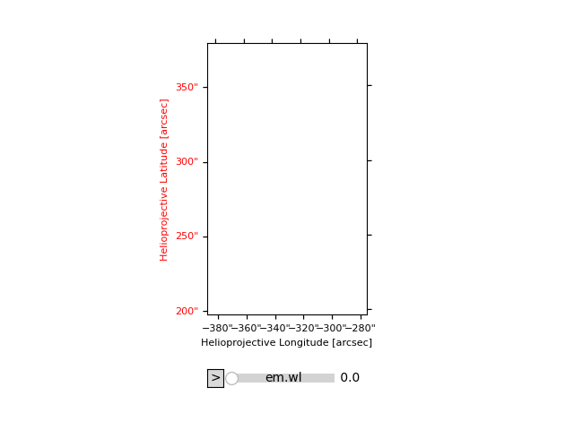
Let’s plot it:
fig = plt.figure()
mg_ii.plot(fig=fig)
<irispy.visualization.IRISArrayAnimatorWCS object at 0x71f3f1421e50>
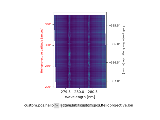
If we want to “raster” over wavelength, we can do the following
This will also “transpose” the data but this is only for visualization purposes We have to set the vmin and vmax, as by default “plot” works out the vmin,vmax from the first slice which in this case is 0.
fig = plt.figure()
mg_ii.plot(fig=fig, plot_axes=["x", "y", None], vmin=0, vmax=1000)
/home/docs/checkouts/readthedocs.org/user_builds/irispy/conda/stable/lib/python3.13/site-packages/ndcube/visualization/mpl_plotter.py:261: NDCubeUserWarning: Animating a NDCube does not support transposing the array. The world axes may not display as expected because the array will not be transposed.
  warn_user(

<irispy.visualization.IRISArrayAnimatorWCS object at 0x71f3d1c5ead0>
This object is sliceable, so we can do things like this:
print(mg_ii[120, 200])
/home/docs/checkouts/readthedocs.org/user_builds/irispy/conda/stable/lib/python3.13/site-packages/astropy/wcs/wcsapi/fitswcs.py:555: AstropyUserWarning: target cannot be converted to ICRS, so will not be set on SpectralCoord
  warnings.warn(

SpectrogramCube
---------------
Obs ID:             3610108077
Obs Description:    Very large dense 320-step raster 105.3x175 320s   Deep x 8 Spatial x
Obs Date:           2018-01-02T15:50:20.710 -- 2018-01-02T15:50:20.710
Data shape:         (380,)
Axis Types:         [('em.wl',)]
Roll:               0.000230473
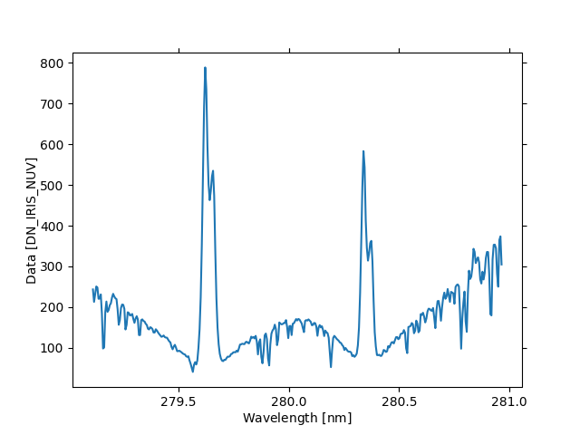
We can also plot this as well, using the WCS information to get the correct axes labels and units.
fig = plt.figure()
ax = fig.add_subplot(111, projection=mg_ii[120, 200].wcs)
# This is just the data values along the wavelength axis of the Mg II k window at pixel (120, 200)
mg_ii[120, 200].plot(axes=ax)
<WCSAxes: ylabel='Data [DN_IRIS_NUV]'>
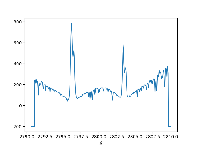
We can also plot using the data directly. We can read the wavelengths of the
Mg window by calling ndcube.NDCube.axis_world_coords for “wl” (wavelength),
and redo the plot.
(mg_wave,) = mg_ii.axis_world_coords("wl")

fig, ax = plt.subplots()
ax.plot(mg_wave.to("AA"), mg_ii.data[120, 200])
/home/docs/checkouts/readthedocs.org/user_builds/irispy/conda/stable/lib/python3.13/site-packages/astropy/wcs/wcsapi/fitswcs.py:555: AstropyUserWarning: target cannot be converted to ICRS, so will not be set on SpectralCoord
  warnings.warn(

[<matplotlib.lines.Line2D object at 0x71f3d1d6f750>]
When we use the underlying data directly, we lose all the metadata and WCS information.
So the main workflow for most code in irispy is to use provided WCS wherever possible
, and only use the underlying data when you need to do some custom processing.
If you are unfamiliar with WCS, the following links are quite useful:
Some of the higher-level utilities are via ndcube, e.g., coordinate transformations: https://docs.sunpy.org/projects/ndcube/en/stable/explaining_ndcube/coordinates.html.
Now, let’s take a look at the WCS information. For example, what is the wavelength position that corresponds to Mg II k core (279.63 nm)?
iris_observer = wcs_to_celestial_frame(mg_ii.wcs.celestial).observer
iris_frame = Helioprojective(observer=iris_observer)
wcs_loc = mg_ii.wcs.world_to_pixel(
    SpectralCoord(279.63, unit=u.nm),
    SkyCoord(0 * u.arcsec, 0 * u.arcsec, frame=iris_frame),
)
mg_index = int(np.round(wcs_loc[0]))
print(mg_index)
/home/docs/checkouts/readthedocs.org/user_builds/irispy/conda/stable/lib/python3.13/site-packages/astropy/wcs/wcsapi/fitswcs.py:555: AstropyUserWarning: target cannot be converted to ICRS, so will not be set on SpectralCoord
  warnings.warn(
/home/docs/checkouts/readthedocs.org/user_builds/irispy/conda/stable/lib/python3.13/site-packages/astropy/wcs/wcsapi/fitswcs.py:723: AstropyUserWarning: No observer defined on WCS, SpectralCoord will be converted without any velocity frame change
  warnings.warn(
111
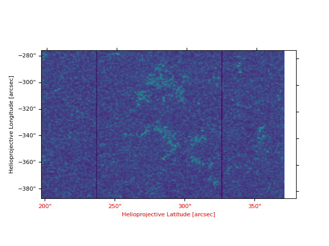
Now we will plot spectroheliogram for Mg II k core wavelength.
We can use the crop method to get this information, this will
require a astropy.coordinates.SpectralCoord object from astropy.coordinates.
# Note that this has to be in axis order and that None, means that the axis is not cropped
lower_corner = [SpectralCoord(280, unit=u.nm), None]
upper_corner = [SpectralCoord(280, unit=u.nm), None]
mg_spec_crop = mg_ii.crop(lower_corner, upper_corner)

fig = plt.figure()
ax = fig.add_subplot(111, projection=mg_spec_crop.wcs)
mg_spec_crop.plot(axes=ax)
<WCSAxes: >
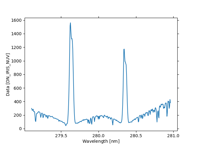
Imagine there’s a really cool feature at (-338”, 275”), how can you plot the spectrum at that location?
lower_corner = [None, SkyCoord(-338 * u.arcsec, 275 * u.arcsec, frame=iris_frame)]
upper_corner = [None, SkyCoord(-338 * u.arcsec, 275 * u.arcsec, frame=iris_frame)]
mg_ii_cut = mg_ii.crop(lower_corner, upper_corner)

fig = plt.figure()
ax = fig.add_subplot(111, projection=mg_ii_cut.wcs)
mg_ii_cut.plot(axes=ax)

plt.show()
/home/docs/checkouts/readthedocs.org/user_builds/irispy/conda/stable/lib/python3.13/site-packages/astropy/wcs/wcsapi/fitswcs.py:555: AstropyUserWarning: target cannot be converted to ICRS, so will not be set on SpectralCoord
  warnings.warn(
Now, you may also be interested in knowing the time that was this observation taken.
There is some information in .meta.
print(mg_ii.meta)
SGMeta
------
Observatory:     IRIS
Instrument:      SPEC
Detector:        NUV
Spectral Window: Mg II k 2796
Spectral Range:  [2790.65477674 2809.95345615] Angstrom
Spectral Band:   NUV
Dimensions:      [320 548 380]
Date:            2018-01-02T15:31:55.870
OBS ID:          3610108077
OBS Description: Very large dense 320-step raster 105.3x175 320s   Deep x 8 Spatial x
But this is mostly about the observation in general. Times of individual scans are saved in .extra_coords[‘time’]. Getting access to it can be done in the following way:
print(mg_ii.axis_world_coords("time", wcs=mg_ii.extra_coords))
(<Time object: scale='utc' format='isot' value=['2018-01-02T15:31:55.870' '2018-01-02T15:32:05.090'
 '2018-01-02T15:32:14.370' '2018-01-02T15:32:23.410'
 '2018-01-02T15:32:32.760' '2018-01-02T15:32:41.930'
 '2018-01-02T15:32:51.210' '2018-01-02T15:33:00.250'
 '2018-01-02T15:33:09.630' '2018-01-02T15:33:18.740'
 '2018-01-02T15:33:28.020' '2018-01-02T15:33:37.050'
 '2018-01-02T15:33:46.410' '2018-01-02T15:33:55.590'
 '2018-01-02T15:34:04.870' '2018-01-02T15:34:13.890'
 '2018-01-02T15:34:23.190' '2018-01-02T15:34:32.400'
 '2018-01-02T15:34:41.680' '2018-01-02T15:34:50.730'
 '2018-01-02T15:35:00.060' '2018-01-02T15:35:09.240'
 '2018-01-02T15:35:18.520' '2018-01-02T15:35:27.530'
 '2018-01-02T15:35:36.850' '2018-01-02T15:35:46.060'
 '2018-01-02T15:35:55.340' '2018-01-02T15:36:04.350'
 '2018-01-02T15:36:13.680' '2018-01-02T15:36:22.900'
 '2018-01-02T15:36:32.180' '2018-01-02T15:36:41.180'
 '2018-01-02T15:36:50.490' '2018-01-02T15:36:59.710'
 '2018-01-02T15:37:08.990' '2018-01-02T15:37:18.010'
 '2018-01-02T15:37:27.340' '2018-01-02T15:37:36.560'
 '2018-01-02T15:37:45.840' '2018-01-02T15:37:54.840'
 '2018-01-02T15:38:04.150' '2018-01-02T15:38:13.370'
 '2018-01-02T15:38:22.650' '2018-01-02T15:38:31.650'
 '2018-01-02T15:38:40.990' '2018-01-02T15:38:50.210'
 '2018-01-02T15:38:59.490' '2018-01-02T15:39:08.490'
 '2018-01-02T15:39:17.810' '2018-01-02T15:39:27.020'
 '2018-01-02T15:39:36.310' '2018-01-02T15:39:45.310'
 '2018-01-02T15:39:54.650' '2018-01-02T15:40:03.870'
 '2018-01-02T15:40:13.150' '2018-01-02T15:40:22.150'
 '2018-01-02T15:40:31.460' '2018-01-02T15:40:40.680'
 '2018-01-02T15:40:49.960' '2018-01-02T15:40:58.960'
 '2018-01-02T15:41:08.310' '2018-01-02T15:41:17.520'
 '2018-01-02T15:41:26.810' '2018-01-02T15:41:35.810'
 '2018-01-02T15:41:45.120' '2018-01-02T15:41:54.340'
 '2018-01-02T15:42:03.620' '2018-01-02T15:42:12.620'
 '2018-01-02T15:42:21.960' '2018-01-02T15:42:31.180'
 '2018-01-02T15:42:40.460' '2018-01-02T15:42:49.460'
 '2018-01-02T15:42:58.770' '2018-01-02T15:43:07.990'
 '2018-01-02T15:43:17.270' '2018-01-02T15:43:26.270'
 '2018-01-02T15:43:35.620' '2018-01-02T15:43:44.840'
 '2018-01-02T15:43:54.120' '2018-01-02T15:44:03.120'
 '2018-01-02T15:44:12.430' '2018-01-02T15:44:21.650'
 '2018-01-02T15:44:30.930' '2018-01-02T15:44:39.930'
 '2018-01-02T15:44:49.270' '2018-01-02T15:44:58.490'
 '2018-01-02T15:45:07.770' '2018-01-02T15:45:16.780'
 '2018-01-02T15:45:26.090' '2018-01-02T15:45:35.310'
 '2018-01-02T15:45:44.590' '2018-01-02T15:45:53.590'
 '2018-01-02T15:46:02.930' '2018-01-02T15:46:12.150'
 '2018-01-02T15:46:21.430' '2018-01-02T15:46:30.430'
 '2018-01-02T15:46:39.740' '2018-01-02T15:46:48.960'
 '2018-01-02T15:46:58.240' '2018-01-02T15:47:07.240'
 '2018-01-02T15:47:16.590' '2018-01-02T15:47:25.810'
 '2018-01-02T15:47:35.090' '2018-01-02T15:47:44.090'
 '2018-01-02T15:47:53.400' '2018-01-02T15:48:02.620'
 '2018-01-02T15:48:11.900' '2018-01-02T15:48:20.900'
 '2018-01-02T15:48:30.240' '2018-01-02T15:48:39.460'
 '2018-01-02T15:48:48.740' '2018-01-02T15:48:57.740'
 '2018-01-02T15:49:07.060' '2018-01-02T15:49:16.270'
 '2018-01-02T15:49:25.560' '2018-01-02T15:49:34.560'
 '2018-01-02T15:49:43.900' '2018-01-02T15:49:53.120'
 '2018-01-02T15:50:02.400' '2018-01-02T15:50:11.400'
 '2018-01-02T15:50:20.710' '2018-01-02T15:50:29.930'
 '2018-01-02T15:50:39.210' '2018-01-02T15:50:48.210'
 '2018-01-02T15:50:57.560' '2018-01-02T15:51:06.770'
 '2018-01-02T15:51:16.060' '2018-01-02T15:51:25.060'
 '2018-01-02T15:51:34.370' '2018-01-02T15:51:43.590'
 '2018-01-02T15:51:52.870' '2018-01-02T15:52:01.870'
 '2018-01-02T15:52:11.210' '2018-01-02T15:52:20.430'
 '2018-01-02T15:52:29.710' '2018-01-02T15:52:38.710'
 '2018-01-02T15:52:48.020' '2018-01-02T15:52:57.240'
 '2018-01-02T15:53:06.520' '2018-01-02T15:53:15.530'
 '2018-01-02T15:53:24.870' '2018-01-02T15:53:34.090'
 '2018-01-02T15:53:43.370' '2018-01-02T15:53:52.370'
 '2018-01-02T15:54:01.680' '2018-01-02T15:54:10.900'
 '2018-01-02T15:54:20.180' '2018-01-02T15:54:29.190'
 '2018-01-02T15:54:38.520' '2018-01-02T15:54:47.740'
 '2018-01-02T15:54:57.020' '2018-01-02T15:55:06.020'
 '2018-01-02T15:55:15.340' '2018-01-02T15:55:24.560'
 '2018-01-02T15:55:33.840' '2018-01-02T15:55:42.840'
 '2018-01-02T15:55:52.180' '2018-01-02T15:56:01.340'
 '2018-01-02T15:56:10.680' '2018-01-02T15:56:19.680'
 '2018-01-02T15:56:28.990' '2018-01-02T15:56:38.210'
 '2018-01-02T15:56:47.490' '2018-01-02T15:56:56.490'
 '2018-01-02T15:57:05.840' '2018-01-02T15:57:15.060'
 '2018-01-02T15:57:24.340' '2018-01-02T15:57:33.340'
 '2018-01-02T15:57:42.650' '2018-01-02T15:57:51.870'
 '2018-01-02T15:58:01.150' '2018-01-02T15:58:10.150'
 '2018-01-02T15:58:19.490' '2018-01-02T15:58:28.710'
 '2018-01-02T15:58:37.990' '2018-01-02T15:58:46.990'
 '2018-01-02T15:58:56.310' '2018-01-02T15:59:05.520'
 '2018-01-02T15:59:14.810' '2018-01-02T15:59:23.810'
 '2018-01-02T15:59:33.150' '2018-01-02T15:59:42.370'
 '2018-01-02T15:59:51.650' '2018-01-02T16:00:00.650'
 '2018-01-02T16:00:09.960' '2018-01-02T16:00:19.180'
 '2018-01-02T16:00:28.460' '2018-01-02T16:00:37.460'
 '2018-01-02T16:00:46.810' '2018-01-02T16:00:56.020'
 '2018-01-02T16:01:05.310' '2018-01-02T16:01:14.310'
 '2018-01-02T16:01:23.620' '2018-01-02T16:01:32.840'
 '2018-01-02T16:01:42.120' '2018-01-02T16:01:51.120'
 '2018-01-02T16:02:00.460' '2018-01-02T16:02:09.680'
 '2018-01-02T16:02:18.960' '2018-01-02T16:02:27.960'
 '2018-01-02T16:02:37.270' '2018-01-02T16:02:46.490'
 '2018-01-02T16:02:55.770' '2018-01-02T16:03:04.770'
 '2018-01-02T16:03:14.120' '2018-01-02T16:03:23.340'
 '2018-01-02T16:03:32.620' '2018-01-02T16:03:41.620'
 '2018-01-02T16:03:50.930' '2018-01-02T16:04:00.150'
 '2018-01-02T16:04:09.430' '2018-01-02T16:04:18.430'
 '2018-01-02T16:04:27.770' '2018-01-02T16:04:36.990'
 '2018-01-02T16:04:46.270' '2018-01-02T16:04:55.270'
 '2018-01-02T16:05:04.590' '2018-01-02T16:05:13.810'
 '2018-01-02T16:05:23.090' '2018-01-02T16:05:32.090'
 '2018-01-02T16:05:41.430' '2018-01-02T16:05:50.650'
 '2018-01-02T16:05:59.930' '2018-01-02T16:06:08.930'
 '2018-01-02T16:06:18.240' '2018-01-02T16:06:27.460'
 '2018-01-02T16:06:36.740' '2018-01-02T16:06:45.740'
 '2018-01-02T16:06:55.090' '2018-01-02T16:07:04.310'
 '2018-01-02T16:07:13.590' '2018-01-02T16:07:22.590'
 '2018-01-02T16:07:31.900' '2018-01-02T16:07:41.120'
 '2018-01-02T16:07:50.400' '2018-01-02T16:07:59.400'
 '2018-01-02T16:08:08.740' '2018-01-02T16:08:17.960'
 '2018-01-02T16:08:27.240' '2018-01-02T16:08:36.250'
 '2018-01-02T16:08:45.560' '2018-01-02T16:08:54.770'
 '2018-01-02T16:09:04.060' '2018-01-02T16:09:13.060'
 '2018-01-02T16:09:22.400' '2018-01-02T16:09:31.620'
 '2018-01-02T16:09:40.900' '2018-01-02T16:09:49.900'
 '2018-01-02T16:09:59.210' '2018-01-02T16:10:08.430'
 '2018-01-02T16:10:17.710' '2018-01-02T16:10:26.710'
 '2018-01-02T16:10:36.060' '2018-01-02T16:10:45.270'
 '2018-01-02T16:10:54.560' '2018-01-02T16:11:03.560'
 '2018-01-02T16:11:12.870' '2018-01-02T16:11:22.090'
 '2018-01-02T16:11:31.370' '2018-01-02T16:11:40.370'
 '2018-01-02T16:11:49.710' '2018-01-02T16:11:58.930'
 '2018-01-02T16:12:08.210' '2018-01-02T16:12:17.210'
 '2018-01-02T16:12:26.520' '2018-01-02T16:12:35.740'
 '2018-01-02T16:12:45.020' '2018-01-02T16:12:54.020'
 '2018-01-02T16:13:03.370' '2018-01-02T16:13:12.590'
 '2018-01-02T16:13:21.870' '2018-01-02T16:13:30.870'
 '2018-01-02T16:13:40.180' '2018-01-02T16:13:49.400'
 '2018-01-02T16:13:58.680' '2018-01-02T16:14:07.680'
 '2018-01-02T16:14:17.020' '2018-01-02T16:14:26.240'
 '2018-01-02T16:14:35.520' '2018-01-02T16:14:44.520'
 '2018-01-02T16:14:53.840' '2018-01-02T16:15:03.060'
 '2018-01-02T16:15:12.340' '2018-01-02T16:15:21.340'
 '2018-01-02T16:15:30.680' '2018-01-02T16:15:39.900'
 '2018-01-02T16:15:49.180' '2018-01-02T16:15:58.180'
 '2018-01-02T16:16:07.490' '2018-01-02T16:16:16.710'
 '2018-01-02T16:16:25.990' '2018-01-02T16:16:34.990'
 '2018-01-02T16:16:44.340' '2018-01-02T16:16:53.560'
 '2018-01-02T16:17:02.840' '2018-01-02T16:17:11.840'
 '2018-01-02T16:17:21.150' '2018-01-02T16:17:30.370'
 '2018-01-02T16:17:39.650' '2018-01-02T16:17:48.650'
 '2018-01-02T16:17:57.990' '2018-01-02T16:18:07.210'
 '2018-01-02T16:18:16.490' '2018-01-02T16:18:25.510'
 '2018-01-02T16:18:34.830' '2018-01-02T16:18:44.020'
 '2018-01-02T16:18:53.310' '2018-01-02T16:19:02.310'
 '2018-01-02T16:19:11.650' '2018-01-02T16:19:20.870'
 '2018-01-02T16:19:30.150' '2018-01-02T16:19:39.160'
 '2018-01-02T16:19:48.470' '2018-01-02T16:19:57.680'
 '2018-01-02T16:20:06.960' '2018-01-02T16:20:15.960'
 '2018-01-02T16:20:25.310' '2018-01-02T16:20:34.520'
 '2018-01-02T16:20:43.810' '2018-01-02T16:20:52.810']>,)
Total running time of the script: (0 minutes 11.230 seconds)