Plot a quick SJI

In this example we will show how to plot a South Pole SJI dataset.

import matplotlib.pyplot as plt
import pooch

from irispy.io import read_files

We start with getting data from the IRIS data archive.

In this case, we will use pooch to keep this example self-contained but you can download the data manually using your browser as well.

You will need to update the path to the data in the next section if you do that.

sji_filename = pooch.retrieve(
    "https://www.lmsal.com/solarsoft/irisa/data/level2_compressed/2023/02/11/20230211_083601_3880012095/iris_l2_20230211_083601_3880012095_SJI_2832_t000.fits.gz",
    known_hash="282595a2c0a5400ef98d1df0172618483dc74b5b56ff16a0f388723363c6f0f1",
)

Downloading data from 'https://www.lmsal.com/solarsoft/irisa/data/level2_compressed/2023/02/11/20230211_083601_3880012095/iris_l2_20230211_083601_3880012095_SJI_2832_t000.fits.gz' to file '/home/docs/.cache/pooch/b74a047a9a5d54358fbd7182c04f3948-iris_l2_20230211_083601_3880012095_SJI_2832_t000.fits.gz'.

We will now open the data using a helper function which is designed to read all files from a single observation.

sji_2832 = read_files(sji_filename)

Printing will give us an overview of the SJI dataset.

print(sji_2832)

SJICube
-------
Observatory:           IRIS
Instrument:            SJI
Bandpass:              2832.0
Obs Date:              2023-02-11T08:37:05.800 -- 2023-02-11T09:09:09.200
Total Frames in Obs:   None
Obs ID:                3880012095
Obs Description:       Very large coarse 64-step raster 126x175 64s   Deep x 30
Axis Types:            [('custom:pos.helioprojective.lon', 'custom:pos.helioprojective.lat', 'time', 'custom:CUSTOM', 'custom:CUSTOM', 'custom:CUSTOM', 'custom:CUSTOM', 'custom:CUSTOM', 'custom:CUSTOM', 'custom:CUSTOM', 'custom:CUSTOM', 'custom:CUSTOM'), ('custom:pos.helioprojective.lon', 'custom:pos.helioprojective.lat'), ('custom:pos.helioprojective.lon', 'custom:pos.helioprojective.lat')]
Roll:                  -0.000393857
Cube dimensions:       (16, 1093, 1776)

We will now plot the IRIS SJI data.

You can also change the axis labels and ticks if you so desire. WCSAxes provides us an API we can use.

# Note that the .get_animation() is used to animate this example and is not required normally.
ax = sji_2832.plot().get_animation()
plt.title(f"IRIS SJI {sji_2832.meta['TWAVE1']}", pad=25)

Once Loop Reflect

Text(0.5, 1.0, 'IRIS SJI 2832.0')

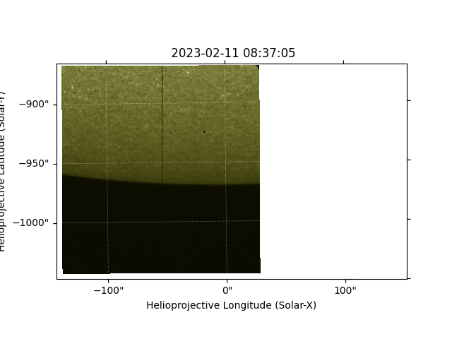
Finally we will output a frame of the SJI into a sunpy Map.

sji_map = sji_2832.to_maps(0)
print(sji_map)

SunPy Map
---------
Observatory:             IRIS
Instrument:              SJI
Detector:
Measurement:             Unknown
Wavelength:              Unknown
Observation Date:        2023-02-11 08:37:05
Exposure Time:           29.9997 s
Dimension:               [1776. 1093.] pix
Coordinate System:       helioprojective
Scale:                   [4.62083333e-05 4.62083333e-05] deg / pix
Reference Pixel:         [887.5 546. ] pix
Reference Coord:         [ 0.00139259 -0.26609909] deg
array([[nan, nan, nan, ..., nan, nan, nan],
       [nan, nan, nan, ..., nan, nan, nan],
       [nan, nan, nan, ..., nan, nan, nan],
       ...,
       [nan, nan, nan, ..., nan, nan, nan],
       [nan, nan, nan, ..., nan, nan, nan],
       [nan, nan, nan, ..., nan, nan, nan]],
      shape=(1093, 1776), dtype=float32)

We can now plot the SJI Map using sunpy Map’s plotting capabilities.

fig = plt.figure()
ax = fig.add_subplot(projection=sji_map.wcs)
sji_map.plot(axes=ax)

plt.show()