Compare Cosmic Ray Removal Backends

This example compares the two cosmic-ray-removal backends supported by irispy:

• rsliding performs sliding sigma clipping (default).

• astroscrappy applies LA Cosmic frame-by-frame.

You can install both optional dependencies with pip install 'irispy-lmsal[cosmic-rays]'.

This example is meant to showcase the difference in one specific case, for a general overview see Remove Cosmic Ray Hits from IRIS data.

import matplotlib.pyplot as plt
import pooch

from astropy.visualization import quantity_support

from irispy.io import read_files

quantity_support()

<astropy.visualization.units.quantity_support.<locals>.MplQuantityConverter object at 0x71f3d3c92510>

We start with getting data from the IRIS data archive.

In this case, we will use pooch to keep this example self-contained but you can download the data manually using your browser as well.

You will need to update the path to the data in the next section if you do that.

raster_filename = pooch.retrieve(
    "https://www.lmsal.com/solarsoft/irisa/data/level2_compressed/2026/02/09/20260209_215233_3602506433/iris_l2_20260209_215233_3602506433_raster.tar.gz",
    known_hash="bad4a3617d0fd04679203951d7db595df196f79b41a3f6f1f71ce0e301486434",
)

We will now open the data using a helper function which is designed to read all files from a single observation.

raster = read_files(raster_filename)
# Open the data and select one Si IV 1403 slice for the comparison.
raster_1403 = raster["Si IV 1403"][10][4]
del raster

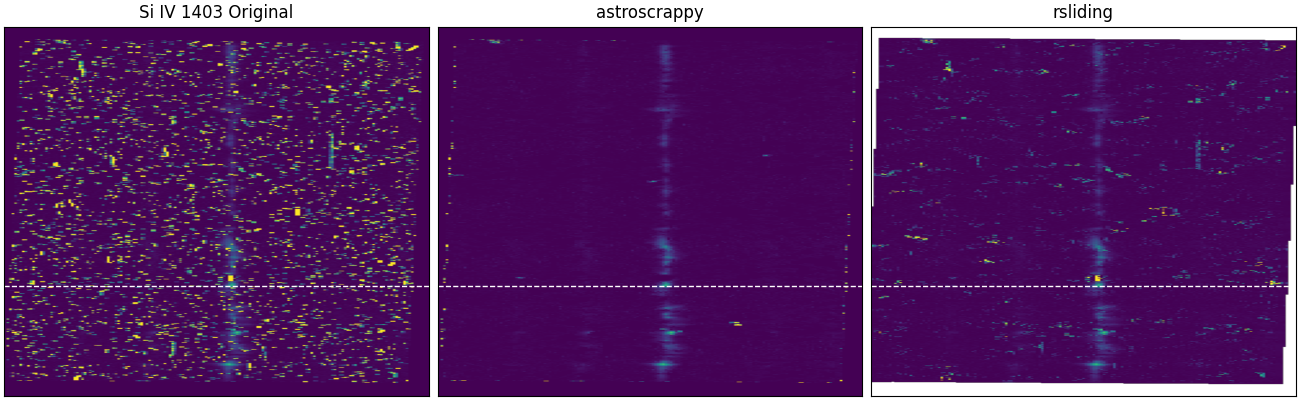
Clean the same Si IV 1403 slice with both supported backends.

astroscrappy is left its backend defaults, while rsliding is given some custom parameters to be more aggressive in fixing spikes.

raster_1403_astroscrappy = raster_1403.remove_cosmic_rays(method="astroscrappy")
raster_1403_rsliding = raster_1403.remove_cosmic_rays(
    method="rsliding",
    sigma=3,
    method_kwargs={
        "kernel": 7,
        "center_choice": "median",
        "borders": "reflect",
        "threads": 1,
    },
)

# This location has a cleaner profile for Si IV 1403.
# If we go to 237, where it looks like we have a strong Si IV 1403,
# it is removed as a spike by both algorithms.
si_iv_idx = 231

fig, axes = plt.subplots(1, 3, figsize=(13, 4), constrained_layout=True)

axes[0].imshow(raster_1403.data, aspect="auto", vmin=0, vmax=500, origin="lower")
axes[0].set_title("Si IV 1403 Original")
axes[1].imshow(raster_1403_astroscrappy.data, aspect="auto", vmin=0, vmax=500, origin="lower")
axes[1].set_title("astroscrappy")
axes[2].imshow(raster_1403_rsliding.data, aspect="auto", vmin=0, vmax=500, origin="lower")
axes[2].set_title("rsliding")

for ax in axes:
    ax.axhline(si_iv_idx, color="white", linestyle="--", linewidth=1)
    ax.set_xlabel("")
    ax.set_ylabel("")
    ax.set_xticks([])
    ax.set_yticks([])

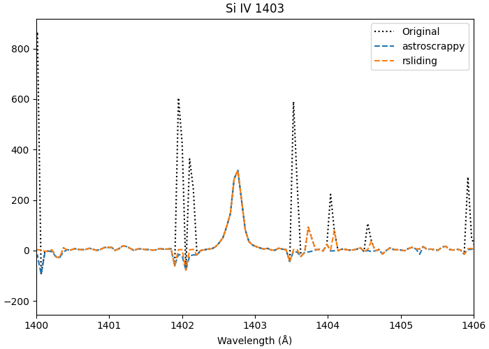
Finally, compare the line profile along the marked row.

si_iv_wave = raster_1403.axis_world_coords("wl")[0].to_value("angstrom")

fig, ax = plt.subplots(1, 1, figsize=(7, 5), constrained_layout=True)
ax.plot(si_iv_wave, raster_1403.data[si_iv_idx, :], label="Original", linestyle="dotted", color="black")
ax.plot(si_iv_wave, raster_1403_astroscrappy.data[si_iv_idx, :], label="astroscrappy", linestyle="dashed")
ax.plot(si_iv_wave, raster_1403_rsliding.data[si_iv_idx, :], label="rsliding", linestyle="dashed")
ax.set_title("Si IV 1403")
ax.set_xlabel("Wavelength (Å)")
ax.set_xlim(1400, 1406)
ax.legend()

/home/docs/checkouts/readthedocs.org/user_builds/irispy/conda/stable/lib/python3.13/site-packages/astropy/wcs/wcsapi/fitswcs.py:555: AstropyUserWarning: target cannot be converted to ICRS, so will not be set on SpectralCoord
  warnings.warn(

<matplotlib.legend.Legend object at 0x71f3d1d6fc50>

In practice, the comparison is not about choosing one universally “better” algorithm. You will need run both, change the parameters, and visually inspect the results to find the best solution for your data and science case.

plt.show()