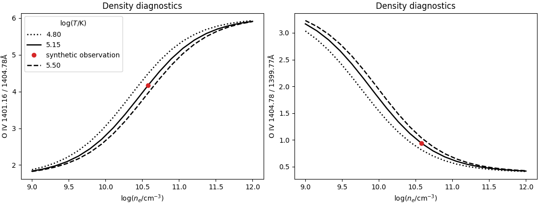
O IV Density-Diagnostic Curves

The goal of this example is to show how to compute and plot density-sensitive O IV line ratios with density_diagnostic. These ratios are sensitive to the electron density in the solar atmosphere, and they are often used to diagnose conditions in the solar transition region.

Warning

This example requires the optional density dependencies, including a version of fiasco that provides fiasco.line_ratio.

import fiasco
import matplotlib.pyplot as plt
import numpy as np

import astropy.units as u

from irispy.utils.density import density_diagnostic

We will reproduce aspects of the top row of Fig. 4 from Dudik et al. (2014), which shows the O IV line ratios as a function of electron density for three different Maxwellian temperatures.

density = np.logspace(9, 12, 20) * u.cm**-3
temperature_samples = 10 ** np.array([4.80, 5.15, 5.50]) * u.K
line_styles = [":", "-", "--"]
temperature_labels = ["4.80", "5.15", "5.50"]
o4_models = []
for temperature, line_style, label in zip(
    temperature_samples,
    line_styles,
    temperature_labels,
    strict=True,
):
    ion = fiasco.Ion("O IV", np.array([temperature.to_value("K")]) * u.K, ask_before=False)
    o4_models.append((line_style, label, ion))

ratio_definitions = [
    ("O IV 1401.16 / 1404.78Å", 1401.157 * u.angstrom, 1404.806 * u.angstrom),
    ("O IV 1404.78 / 1399.77Å", 1404.806 * u.angstrom, 1399.780 * u.angstrom),
]

The exact curve values will differ somewhat from the paper because this example uses the current CHIANTI database through fiasco rather than the CHIANTI version used by Dudik et al. (2014).

# `~irispy.utils.density.density_diagnostic` needs measured line intensities as
# input because it maps an observed ratio back to density. To plot the diagnostic
# curves, we first use unit intensities and then use one point on the returned
# curve as a synthetic observation.

fig, axes = plt.subplots(
    ncols=2,
    figsize=(11, 4.2),
    constrained_layout=True,
    sharex=True,
)

line_ratio_kwargs = {"use_two_ion_model": False}
for ax, (title, numerator, denominator) in zip(axes, ratio_definitions, strict=True):
    for line_style, label, ion in o4_models:
        diagnostic = density_diagnostic(
            1 * u.ct,
            1 * u.ct,
            density,
            ion=ion,
            numerator=numerator,
            denominator=denominator,
            temperature=ion.temperature,
            line_ratio_kwargs=line_ratio_kwargs,
        )
        ax.plot(
            np.log10(diagnostic["density_grid"].to_value("cm-3")),
            diagnostic["theoretical_ratio"].value,
            color="black",
            linestyle=line_style,
            linewidth=1.8,
            label=label,
        )
        if label == "5.15":
            sample_index = diagnostic["density_grid"].size // 2
            sample_ratio = diagnostic["theoretical_ratio"][sample_index]
            observed = density_diagnostic(
                sample_ratio.value * 100 * u.ct,
                100 * u.ct,
                density,
                ion=ion,
                numerator=numerator,
                denominator=denominator,
                temperature=ion.temperature,
                line_ratio_kwargs=line_ratio_kwargs,
            )
            ax.plot(
                np.log10(observed["density"].to_value("cm-3")),
                observed["ratio"].value,
                color="tab:red",
                marker="o",
                linestyle="none",
                label="synthetic observation" if ax is axes[0] else None,
            )
    ax.set_title("Density diagnostics")
    ax.set_xlabel(r"$\log(n_e / \mathrm{cm^{-3}})$")
    ax.set_ylabel(title)

axes[0].legend(loc="upper left", title=r"$\log(T / \mathrm{K})$")

plt.show()