Apply Radiometric Calibration

In this example we will show how to perform radiometric calibration on IRIS data.

IRIS level 2 data are provided in units of Data Number (DN). To convert these to a flux in physical units (e.g., \(erg s^{-1} sr^{-1} cm^{-2} Å^{-1}\)) one must perform a radiometric calibration.

The calibration output has been confirmed to provide the same results as those provided by the SolarSoft IDL routine IRIS_CALIB.

The major difference being that the output here is accounting for the wavelength, which is why the units here are \(erg s^{-1} sr^{-1} cm^{-2} Å^{-1}\) and not \(erg s^{-1} sr^{-1} cm^{-2}\). Notice the extra \(Å^{-1}\) in the units.

Please refer to ITN26 for more information on the calibration process.

import matplotlib.pyplot as plt
import pooch

import astropy.units as u

from irispy.io import read_files
from irispy.utils.spectrograph import radiometric_calibration

We start with getting data from the IRIS data archive.

In this case, we will use pooch to keep this example self-contained but you can download the data manually using your browser as well.

You will need to update the path to the data in the next section if you do that.

raster_filename = pooch.retrieve(
    "https://www.lmsal.com/solarsoft/irisa/data/level2_compressed/2026/03/08/20260308_051050_3893012099/iris_l2_20260308_051050_3893012099_raster.tar.gz",
    known_hash="b76277ae89e79f50e7ddc603a86b9bbf70e23b2e64fc5343dbe99af19a05f854",
)

We will now open the data using a helper function which is designed to read all files from a single observation.

raster = read_files(raster_filename)

We will just focus on the Mg II k 2796 line which we can select using a key. Then we will just plot a spectral line selected at random in space.

# There is only one complete scan, so we index that away.
# We also only take the first scan of the sequence to reduce memory usage for
# the online documentation build.
mg_ii_k_2796 = raster["Mg II k 2796"][0][0]
del raster

To convert the spectral units from DN to flux one must do the following calculation:

\[\mathrm{Flux}(\mathrm{erg}\: \mathrm{s}^{-1}\: \mathrm{cm}^{-2} \text{Å}^{-1}\: \mathrm{sr}^{-1}) = \mathrm{Flux}(\mathrm{DN}) \frac{E_\lambda \cdot \mathrm{DN2PHOT\_SG}}{A_\mathrm{eff} \cdot \mathrm{Pix}_{xy} \cdot \mathrm{Pix}_{\lambda} \cdot t_\mathrm{exp} \cdot W_\mathrm{slit}},\]

where \(E_\lambda \equiv h \cdot c / \lambda\) is the photon energy (in erg), \(DN2PHOT\_SG\) is the number of photons per DN, \(A_\mathrm{eff}\) is the effective area (in \(cm^{-2}\)), \(Pix_{xy}\) is the size of the spatial pixels in radians (e.g., multiply the spatial binning factor by \(\pi/(180\cdot3600\cdot6)\)), \(Pix_{\lambda}\) is the size of the spectral pixels in \(Å\), \(t_\mathrm{exp}\) is the exposure time in seconds and \(W_\mathrm{slit}\) is the slit width in radians (\(W_\mathrm{slit} \equiv \pi/(180\cdot3600\cdot3)\)).

This is a complex equation and requires careful attention to units. Within irispy, there is a function called irispy.utils.spectrograph.radiometric_calibration that handles this process.

calibrated_mg_ii_k_2796 = radiometric_calibration(mg_ii_k_2796)

/home/docs/checkouts/readthedocs.org/user_builds/irispy/conda/stable/lib/python3.13/site-packages/astropy/wcs/wcsapi/fitswcs.py:555: AstropyUserWarning: target cannot be converted to ICRS, so will not be set on SpectralCoord
  warnings.warn(
/home/docs/checkouts/readthedocs.org/user_builds/irispy/conda/stable/lib/python3.13/site-packages/erfa/core.py:133: ErfaWarning: ERFA function "utctai" yielded 1 of "dubious year (Note 3)"
  warn(f'ERFA function "{func_name}" yielded {wmsg}', ErfaWarning)

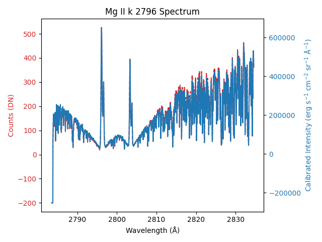
We will now plot both the before and after spectrums at a single spatial pixel to see the difference.

fig, ax = plt.subplots()
color = "tab:red"
ax.set_xlabel("Wavelength (Å)")
ax.set_ylabel("Counts (DN)", color=color)
ax.plot(
    mg_ii_k_2796.spectral_axis[10:-20].to(u.angstrom),
    mg_ii_k_2796.data[100, 10:-20],
    color=color,
    linestyle="dashed",
)
ax.tick_params(axis="y", labelcolor=color)

ax2 = ax.twinx()

color = "tab:blue"
ax2.plot(
    calibrated_mg_ii_k_2796.spectral_axis[10:-20].to(u.angstrom),
    calibrated_mg_ii_k_2796.data[100, 10:-20],
    color=color,
)
ax2.set_ylabel("Calibrated Intensity (erg s$^{-1}$ cm$^{-2}$ sr$^{-1}$ Å$^{-1}$)", color=color)
ax2.tick_params(axis="y", labelcolor=color)

ax.set_title("Mg II k 2796 Spectrum")
fig.tight_layout()

plt.show()

/home/docs/checkouts/readthedocs.org/user_builds/irispy/conda/stable/lib/python3.13/site-packages/astropy/wcs/wcsapi/fitswcs.py:555: AstropyUserWarning: target cannot be converted to ICRS, so will not be set on SpectralCoord
  warnings.warn(