Compare SJI and SG slit coordinates

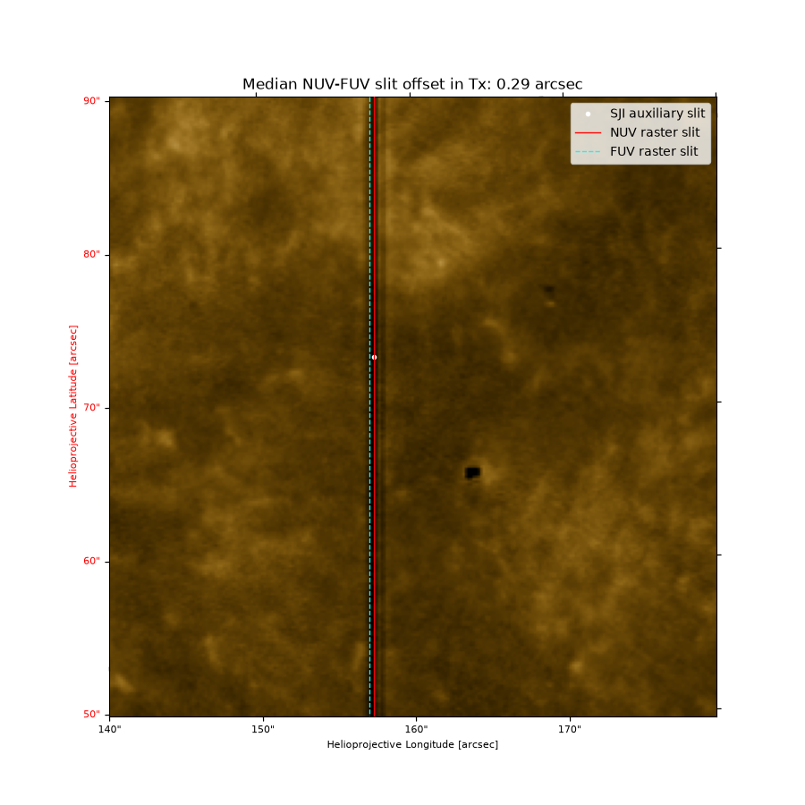
This example compares the slit location recorded with an IRIS 2796 slit-jaw imager (SJI) with the slit coordinates from matching NUV and FUV spectrograph (SG) raster steps.

import matplotlib.pyplot as plt
import numpy as np
import pooch

import astropy.units as u
from astropy.coordinates import SkyCoord
from astropy.io import fits
from astropy.visualization import time_support
from astropy.wcs.utils import wcs_to_celestial_frame

from irispy.io import read_files

time_support()

<astropy.visualization.time.time_support.<locals>.MplTimeConverter object at 0x7a90a11e2a50>

We will start by getting some data from the IRIS archive.

In this case, we will use pooch so to keep this example self-contained but using your browser will also work.

Using the url: https://www.lmsal.com/hek/hcr?cmd=view-event&event-id=ivo%3A%2F%2Fsot.lmsal.com%2FVOEvent%23VOEvent_IRIS_20130902_182935_4000005156_2013-09-02T18%3A29%3A352013-09-02T18%3A29%3A35.xml we are after the 2796 slit-jaw images and the raster sequence.

raster_filename = pooch.retrieve(
    "https://www.lmsal.com/solarsoft/irisa/data/level2_compressed/2013/09/02/20130902_182935_4000005156/iris_l2_20130902_182935_4000005156_raster.tar.gz",
    known_hash="91211a52e278fb6e535242d4d6064facf9f93cf24f0a433c276ace1b2d621e7d",
)
sji_filename = pooch.retrieve(
    "https://www.lmsal.com/solarsoft/irisa/data/level2_compressed/2013/09/02/20130902_182935_4000005156/iris_l2_20130902_182935_4000005156_SJI_2796_t000_deconvolved.fits.gz",
    known_hash="2043c85e567a5a0ad8cf9024745dae87f632d5c4cd019cc0e7bfeb7a1fae99d0",
)

Now to open the files using irispy.

raster = read_files(raster_filename)
sji_2796 = read_files(sji_filename)

Now we will find the closest SJI time to the 56th raster step.

# The pointing correction is detector-specific, so compare the NUV SJI with an
# NUV spectrograph window rather than, for example, the FUV C II window.
mg_ii = raster["Mg II k 2796"][0]
c_ii = raster["C II 1336"][0]

times_SG = mg_ii.axis_world_coords("time", wcs=mg_ii.extra_coords)
(time_2796,) = sji_2796.axis_world_coords("time")
# We picked randomly.
raster_idx = 55
time_target = times_SG[0][raster_idx]

time_idx_2796 = np.abs(time_2796 - time_target).argmin()
time_stamp_2796 = time_2796[time_idx_2796].isot
print(time_stamp_2796, "\n", time_target, "\n", time_idx_2796)

2013-09-02T18:32:16.310
 2013-09-02T18:32:16.380
 13

We will require the slit location from the SJI auxiliary data later on.

with fits.open(sji_filename) as sji_hdulist:
    sji_aux_header = sji_hdulist[-2].header
    sji_aux_data = sji_hdulist[-2].data
    # Use the header-provided column indices instead of relying on fixed array columns.
    sji_slit_location_pixel_x = sji_aux_data[time_idx_2796, sji_aux_header["SLTPX1IX"]]
    sji_slit_location_pixel_y = sji_aux_data[time_idx_2796, sji_aux_header["SLTPX2IX"]]

The POFFY* auxiliary values are offsets in spatial pixels. If they need to be converted manually, multiply each value by CDELT2 from the same data product. CDELT2 includes spatial summing; the physical slit width does not. irispy already applies the detector-specific spectograph correction when reading the raster, so applying an auxiliary offset again here would double-correct the WCS.

We can now get the slit locations from the raster FITS WCSes.

sji_2796_closest = sji_2796[time_idx_2796]
sji_2796_frame = wcs_to_celestial_frame(sji_2796_closest.basic_wcs)

nuv_lon_coords = mg_ii.axis_world_coords_values("custom:pos.helioprojective.lon")[0][raster_idx]
nuv_lat_coords = mg_ii.axis_world_coords_values("custom:pos.helioprojective.lat")[0][raster_idx]
fuv_lon_coords = c_ii.axis_world_coords_values("custom:pos.helioprojective.lon")[0][raster_idx]
fuv_lat_coords = c_ii.axis_world_coords_values("custom:pos.helioprojective.lat")[0][raster_idx]

The FUV and NUV spectrographs share one physical slit, but use separate detectors whose fiducial positions and pointing corrections are tracked independently. Their WCS slit coordinates have a detector-dependent offset in this observation.

nuv_slit = SkyCoord(Tx=nuv_lon_coords, Ty=nuv_lat_coords, frame=sji_2796_frame)
fuv_slit = SkyCoord(Tx=fuv_lon_coords, Ty=fuv_lat_coords, frame=sji_2796_frame)
nuv_fuv_slit_separation = np.nanmedian(np.abs(nuv_slit.Tx - fuv_slit.Tx)).to(u.arcsec)

Now we can compare the locations and make sure they match.

fig = plt.figure(figsize=(9, 9))
ax = fig.add_subplot(projection=sji_2796_closest)
sji_2796_closest.plot(ax)

# This is the pixel location of the slit in the SJI data based on the auxiliary data.
slit_location_from_sji_aux = sji_2796[time_idx_2796].wcs.pixel_to_world(
    sji_slit_location_pixel_x, sji_slit_location_pixel_y
)
ax.plot_coord(slit_location_from_sji_aux, ".", color="white", label="SJI auxiliary slit")

# These are the matching NUV and FUV raster slit coordinates from their FITS WCSes.
ax.plot_coord(nuv_slit, color="red", linestyle="-", linewidth=1, label="NUV raster slit")
ax.plot_coord(fuv_slit, color="cyan", linestyle="--", linewidth=1, label="FUV raster slit")
ax.set_title(f"Median NUV-FUV slit offset in Tx: {nuv_fuv_slit_separation:.2f}")
ax.legend()

# "Crop" the image without touching the actual data.
bbox = SkyCoord([140, 180] * u.arcsec, [50, 90] * u.arcsec, frame=sji_2796_frame)
x_limit, y_limit = sji_2796_closest.wcs.world_to_pixel(bbox)
ax.set_xlim(int(x_limit[0]), int(x_limit[1]))
ax.set_ylim(int(y_limit[0]), int(y_limit[1]))

plt.show()