Calculate Red-Blue Asymmetry

This example shows how to calculate the Red-Blue Asymmetry (RBA) for an IRIS raster.

RBA is a model-independent metric that compares excess emission in the red and blue wings of a spectral line:

• Positive RBA -> excess red-wing emission

• Negative RBA -> excess blue-wing emission

import matplotlib.pyplot as plt
import numpy as np
import pooch

import astropy.units as u
from astropy.visualization import time_support

from irispy.io import read_files
from irispy.utils.red_blue import RBAQualityFlag, calculate_red_blue_asymmetry

time_support()

<astropy.visualization.time.time_support.<locals>.MplTimeConverter object at 0x7a9099b04d70>

We start with getting data from the IRIS data archive.

In this case, we will use pooch to keep this example self-contained but you can download the data manually using your browser as well.

You will need to update the path to the data in the next section if you do that.

raster_filename = pooch.retrieve(
    "https://www.lmsal.com/solarsoft/irisa/data/level2_compressed/2021/04/29/20210429_110908_3660259102/iris_l2_20210429_110908_3660259102_raster.tar.gz",
    known_hash="6d07f8dfa4c4644f26dce0c63166d22900d263d555c3d142454ff27fe257688b",
)

We will now open the data using a helper function which is designed to read all files from a single observation.

raster = read_files(raster_filename, spectral_windows="Si IV 1403")
# We are after the Si IV 1403 line, which we can select using a key.
si_iv = raster["Si IV 1403"][0]

Now we will calculate the red-blue asymmetry on a small cutout around the selected feature. This keeps the example light enough for documentation builds while still showing the full workflow.

full_raster_pixel_index = (499, 148)
raster_cutout = slice(450, 550)
slit_cutout = slice(100, 200)
si_iv = si_iv[raster_cutout, slit_cutout, :]
selected_pixel_index = (
    full_raster_pixel_index[0] - raster_cutout.start,
    full_raster_pixel_index[1] - slit_cutout.start,
)

si_iv_rest = 140.277 * u.nm
velocity_range = (25, 75) * u.km / u.s
# Ignore pixels where the line peak is too weak for a useful wing comparison.
min_intensity = 75 * si_iv.unit

# rest_wavelength is auto-detected from the cube metadata (TWAVE[N] FITS keyword).
# You can also pass it explicitly: rest_wavelength=si_iv_rest.
red_blue = calculate_red_blue_asymmetry(
    si_iv,
    velocity_range=velocity_range,
    min_intensity=min_intensity,
    return_profiles=True,
)

asymmetry = red_blue["red_blue_asymmetry"]
quality = red_blue["quality"]
observed_profiles = red_blue["observed_profile"]

/home/docs/checkouts/readthedocs.org/user_builds/irispy/conda/latest/lib/python3.13/site-packages/astropy/wcs/wcsapi/fitswcs.py:567: AstropyUserWarning: target cannot be converted to ICRS, so will not be set on SpectralCoord
  warnings.warn(

We add specific metadata to the fitted profiles. This is stored in the meta attribute for each result.

print(asymmetry.meta)

SGMeta
------
Observatory:     IRIS
Instrument:      SPEC
Detector:        FUV2
Spectral Window: Si IV 1403
Spectral Range:  [1398.58006787 1406.74630787] Angstrom
Spectral Band:   FUV
Dimensions:      [100 100]
Date:            2021-04-29T11:09:08.560
OBS ID:          3660259102
OBS Description: Medium sit-and-stare 0.3x60 1s  C II   Si IV   Mg II h/k Deep x 8  F

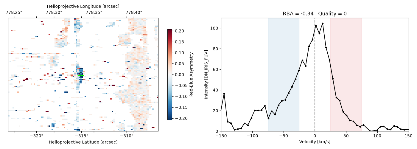
Now we will select a pixel with a significant red excess (positive RBA).

observed_profile = observed_profiles[selected_pixel_index]
velocities = observed_profile.axis_world_coords(0)[0].to(u.km / u.s)
profile = observed_profile.data

Now we will plot the RBA map for the raster and the raw profile in velocity space for the selected pixel.

fig = plt.figure(figsize=(14, 5))
axes = [
    fig.add_subplot(1, 2, 1, projection=asymmetry.wcs),
    fig.add_subplot(1, 2, 2),
]

# This plot will be the RBA values over the full raster.
ax = axes[0]
rba_map = np.where(quality.data == int(RBAQualityFlag.OK), asymmetry.data, np.nan)
# Colour scale: 98th percentile of absolute RBA, floored so subtle features remain visible.
vmax = max(np.nanpercentile(np.abs(rba_map), 98), 0.15)
im = ax.imshow(rba_map, cmap="RdBu_r", origin="lower", aspect="auto", vmin=-vmax, vmax=vmax)
ax.plot(
    selected_pixel_index[1],
    selected_pixel_index[0],
    color="lime",
    marker="+",
    linestyle="none",
    markersize=16,
    transform=ax.get_transform("pixel"),
)
ax.coords[0].set_axislabel("Helioprojective Latitude [arcsec]")
ax.coords[1].set_axislabel("Helioprojective Longitude [arcsec]")
fig.colorbar(im, ax=ax, shrink=0.8, label="Red-Blue Asymmetry")

# This plot will be the raw profile for the selected pixel.
ax = axes[1]
finite = np.isfinite(velocities.value) & np.isfinite(profile)
ax.plot(velocities.value[finite], profile[finite], color="black", marker="o", markersize=3)
ax.axvline(0, color="grey", linestyle="dashed")

v_low = velocity_range[0].to_value(u.km / u.s)
v_high = velocity_range[1].to_value(u.km / u.s)
ax.axvspan(-v_high, -v_low, color="C0", alpha=0.1)
ax.axvspan(v_low, v_high, color="C3", alpha=0.1)

ax.set_title(
    f"RBA = {float(asymmetry.data[selected_pixel_index]):.2f}   Quality = {int(quality.data[selected_pixel_index]):d}"
)
ax.set_xlabel("Velocity [km/s]")
ax.set_ylabel(f"Intensity [{si_iv.unit.to_string()}]")
ax.set_xlim(-150, 150)
ax.set_ylim(bottom=0)

fig.tight_layout()

plt.show()