Remove Cosmic Rays from IRIS SG data

This example illustrates how to remove cosmic ray hits from IRIS spectrograph data.

We will use rsliding backend, which has to be installed separately using pip or conda. We select rsliding for the SG data because it is considered the better solution for spectral data.

To understand rsliding, how it works and what are allowed parameters, we suggest you read the original documentation:

• rsliding documentation

import matplotlib.pyplot as plt
import pooch

from astropy.visualization import quantity_support

from irispy.io import read_files

quantity_support()

<astropy.visualization.units.quantity_support.<locals>.MplQuantityConverterFormatted object at 0x7a90b4016e40>

We start with getting data from the IRIS data archive.

This dataset is during the South Atlantic Anomaly (SAA) passage, which is known to cause a large number of cosmic ray hits in the data.

This is what we call, a worst-case scenario for cosmic ray removal, which is good for testing the algorithms but not ideal for science.

In this case, we will use pooch to keep this example self-contained but you can download the data manually using your browser as well.

You will need to update the path to the data in the next section if you do that.

raster_filename = pooch.retrieve(
    "https://www.lmsal.com/solarsoft/irisa/data/level2_compressed/2026/02/09/20260209_215233_3602506433/iris_l2_20260209_215233_3602506433_raster.tar.gz",
    known_hash="bad4a3617d0fd04679203951d7db595df196f79b41a3f6f1f71ce0e301486434",
)

We will now open the data using a helper function which is designed to read all files from a single observation.

raster = read_files(raster_filename, spectral_windows="Si IV 1403")
# Open the data and select one slice for the comparison.
raster = raster["Si IV 1403"][10][4]

Now we use remove_cosmic_rays with the default parameters on IRIS Level 2 spectrograph data.

rsliding is the default backend, which is used by the SPICE team for their cosmic ray removal.

rsliding has a set of default parameters that are not necessarily optimal for IRIS data. In addition, there is a lot of optional parameters that can be tweaked, which might improve the results for your data and science case or make it worse. Unfortunately, there is no one-size-fits-all solution for cosmic ray removal, and you will need to read the documentation and experiment with the parameters to find the best solution for your data.

What we can say that is for rsliding, the main parameter to change is the kernel size, which controls how aggressive the algorithm is in removing spikes. The size will depend on the spectral resolution of the data.

# A few other notes about ``rsliding``:
#
# ``rsliding`` seems to perform better on spectra, with the key controlling argument being
# "kernel" and the values found to work the best assuming ~0.0254 :math:`\AA` spectral resolution
#  are 3 and 5.
#
# * 5 is more aggressive, effectively detecting and replacing most of the spikes. A slight
#   disadvantage is that it sometimes designates "real" jumps in the continuum as "spikes" and
#   replaces them.
#
# * 3 works the opposite, it can ignore some real spikes but is less forgiving to the
# irregularities in the continuum. This is also the default value used by ``rsliding``.
#
# One more parameter you might look for is "threads" which controls how much of the CPU is used
# for the despiking. The despiking should take few minutes to run on a cropped intensity cube.

# For example, these set of parameters was shown to show better treatment of values around
# any spikes, basically to smooth more around each spike. (Thanks to Juraj).
method_kwargs = {"kernel": 5, "center_choice": "median", "borders": "reflect"}
raster_rsliding = raster.remove_cosmic_rays(method="rsliding", sigma=3, method_kwargs=method_kwargs)

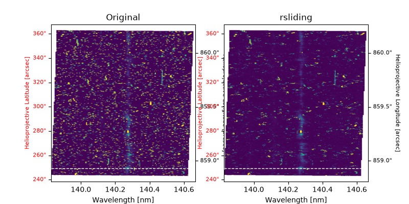
One reason to always be cautious when removing cosmic rays is that you can easily remove real features in the data if you are too aggressive. For example, in this case, we have a strong Si IV 1403 line at around row 246, which is removed as a spike. But we will look at a different row instead, which has a cleaner profile for Si IV 1403.

si_iv_idx = 66

fig, axes = plt.subplots(1, 2, figsize=(8, 4), subplot_kw={"projection": raster.wcs})

raster.plot(axes=axes[0], aspect="auto", vmin=0, vmax=500)
axes[0].set_title("Original")
raster_rsliding.plot(axes=axes[1], aspect="auto", vmin=0, vmax=500)
axes[1].set_title("rsliding")

for ax in axes:
    ax.axhline(si_iv_idx, color="white", linestyle="--", linewidth=1)

/home/docs/checkouts/readthedocs.org/user_builds/irispy/conda/latest/lib/python3.13/site-packages/astropy/wcs/wcsapi/fitswcs.py:567: AstropyUserWarning: target cannot be converted to ICRS, so will not be set on SpectralCoord
  warnings.warn(

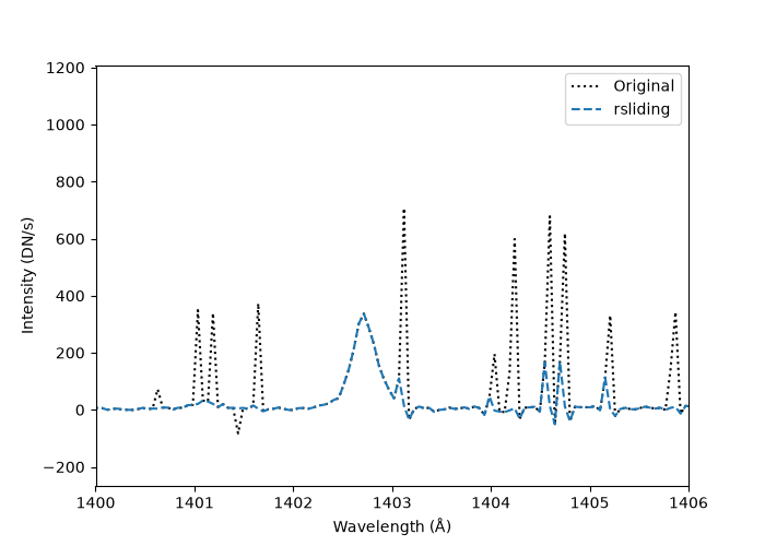
Finally, compare the line profile along the marked row.

si_iv_wave = raster.axis_world_coords("wl")[0].to_value("angstrom")

fig, ax = plt.subplots(1, 1, figsize=(7, 5))
ax.plot(si_iv_wave, raster.data[si_iv_idx, :], label="Original", linestyle="dotted", color="black")
ax.plot(si_iv_wave, raster_rsliding.data[si_iv_idx, :], label="rsliding", linestyle="dashed")
ax.set_ylabel("Intensity (DN/s)")
ax.set_xlabel("Wavelength (Å)")
ax.set_xlim(1400, 1406)
ax.legend()

plt.show()